
To ensure the safety of the people and environment surrounding power lines, the electric and magnetic fields they create must be monitored. Engineers can use modeling and simulation to predict how these fields will spread out from the power lines and how that affects their strength at ground level. Let’s take a look at two examples of how the COMSOL Multiphysics® software can be used to analyze these fields generated from power lines.
Invisible Localities of Energy
Much of the everyday electricity that we use is sourced from high to low voltage power lines, which create both electric and magnetic fields (EMFs). Power lines conduct strong low-frequency currents, giving rise to nonionizing EMFs that fade quickly with distance. Still, it is important to monitor both the exposure and output of these fields to ensure that they stay within a safe range for the surrounding individuals and environment.
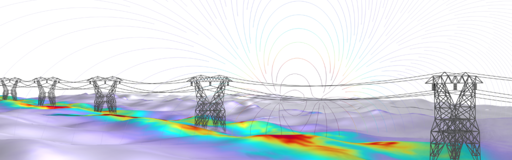
Figure 1. A model illustrating power lines sending electricity over long distances.
Next, we’ll explore two examples showcasing the use of modeling and simulation for analyzing the electric and magnetic fields produced by power lines. These examples will focus on the strength of the fields and their distribution in relation to the power lines and towers.
Exploring the Setup of Two Power Line Models
The Electric Field from Power Lines and Magnetic Field from Power Lines models, available in our Application Gallery, feature two towers that transmit high voltage three-phase AC power. The towers are equipped with two shielding lines above the phase lines to prevent damage from lightning strikes. Phase lines are typically made up of several smaller conductors bundled together in transmission lines with such a high voltage. To keep things simple in the models, each phase line uses only one conductor with the radius expanded to 10 cm to mimic that of a bundled conductor. In each model, the ground level is set as a randomly perturbed surface to simulate the irregularities of the earth.
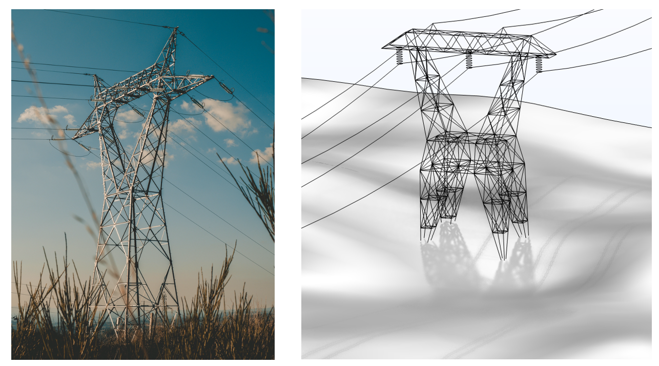
Figure 2. At left: A power line, photo by David Levêque on Unsplash. At right: The geometry of the transmission tower. The two shielding lines can be seen on top, while the three phase lines are held by the insulators.
Now that we’ve covered the basics of both models’ geometries, let’s take a look at the results for each. (Note that the step-by-step instructions for building these models and their MPH-files can be downloaded from their Application Gallery entries, linked at the bottom of this blog post.)
Electric Fields Model
In the electric fields model, users can set the voltage amplitude and phase on each phase line. (In the scenario shown in Figure 3, the voltage was set to 400 kV and the phases were separated by 120º.) In addition, the boundary element method and a fixed potential at all of the edges and surfaces is used, so the model needs a mesh only on these entities. In contrast, the finite element method, where the model would need to create a volumetric mesh in the entire air domain, would drastically increase the number of degrees of freedom and lengthen the time required to solve the model.
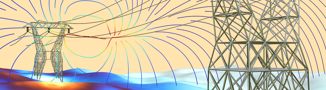
The results show the electric field norm generated from the wires at ground level and the streamlines indicating the local direction of the field in the air. In relation to the power lines, the electric field creates a branching figure. The field is strongest close to the power lines and decreases with distance. Knowing how far the fields spread can help engineers determine how close buildings can be constructed to power lines to minimize exposure and ensure compliance with regulations.

Figure 3. The electric field norm (surface) and the electric field (streamlines) from the transmission lines.
Magnetic Fields Model
In the magnetic fields model, each phase line conducts a 1000 A current. Like the electric fields model, the phases in this model are also separated by 120º. A default magnetic insulation boundary condition is applied to all exterior boundaries in the model.
Also like the electric fields model, the results of the magnetic fields model also shows the magnetic field norm generated from the power line wires at ground level, with streamlines showing the direction of the field. The streamlines form closed loops. The magnetic field in this model is also strongest close to the power lines and decreases with distance.

Figure 4. The magnetic field norm (surface) and the magnetic field (streamlines) from the transmission lines.
Next Steps
In this blog post, we’ve discussed two examples of models that can be built in COMSOL Multiphysics® for examining electric and magnetic field distributions produced by power lines. Models like these are important in measuring the range and behavior of EMFs, which can lead to a further understanding of how EMFs interact with the surrounding environment.
Want to try modeling EMFs from power lines yourself? The models discussed above and their step-by-step instructions are available here:
Further Reading
Read more about simulation’s role in studying EMF exposure on the COMSOL Blog:

Comments (1)
Helger van Halewijn
July 13, 2024Dear Elsa,
Your model setup looks really nice! I am involved in the simulation of magnetic fields in the Netherlands and apply this with 2D models. I use infinite element domains I and I suggest you to take this into account. I am not sure if the behavior of the B-fields are correct at the far outside of your model (It will not influence the field strength very much around the wires)
My 2D models have been verified by a governmental authority and I am on a list with only a few other companies in the Netherlands who are allowed to perform these simulations. It is necessary to know the 0.4 microTesla zone. If buildings or projects are planned for permanent living we have to proof to the local authorities that the planned buildings are outside the 0.4 microTesla level. This has to do with health issues.
If you would like to know more about this, please do not hesitate contacting me. I am more than happy to comment on this subject.
I appreciate your comments,
Regards,
Helger van Halewijn.
Certified Consultant.