

Jan Czochralski was examining the rate at which metals crystallize when he placed a full, hot crucible of molten tin on his desk to cool. Focused on his work, he accidentally sunk his pen into the molten tin instead of the inkwell. Noticing his mistake, Czochralski pulled the pen out — only to discover a thin thread of solidified metal hanging from its tip…
The History Behind the Czochralski Method
Czochralski later proved this solidified metal to be a single crystal. Nearly 110 years later, we recognize that his simple mistake laid the foundation for the Czochralski method, one of the most important methods for the preparation of monocrystalline silicon, a material widely used in the creation of electronics.
Today, the Czochralski method follows a similar process to that accidental dipping of the pen. First, high-purity, semiconductor-grade silicon is melted in a crucible. Next, dopant impurity atoms can be added to dope the silicon and change it into a positive or negative type silicon. Then a rod-mounted seed crystal is dipped into the molten mix and carefully pulled upwards and rotated simultaneously in an inert atmosphere of argon. Finally, a large, single-crystal, cylindrical ingot is formed from the melt.
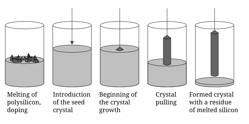 The Czochralski method broken down into stages. This photograph is in the public domain, via Wikimedia Commons.
Czochralski explored this approach to crystal creation with metals such as tin, lead, and zinc and published his paper on the method in 1917. The paper and method had peaked interest upon publication, but it was not until the late 1940s that it became the phenomenon it is today. This is largely thanks to the researchers at Bell Labs who rediscovered this method and used it to produce silicon and germanium crystals in order to develop semiconductors. Since then, the Czochralski method has become a cornerstone in the semiconductor industry.
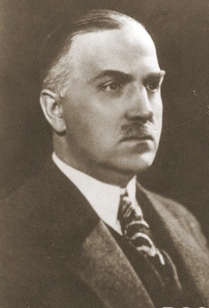
The Polish chemist, Jan Czochralski, as he appeared in 1929 as a professor at Warsaw Polytechnic. This photograph is in the public domain, via Wikimedia Commons.
Czochralski’s method is the most common approach for the preparation of monocrystalline silicon (mono-Si) crystal ingots. This method has produced crystal ingots up to 2 meters in length, which can then be sliced into wafers of standardized dimensions. These are used for the fabrication of integrated circuits and, in photovoltaics, to manufacture solar cells. In this blog post, we will explore how the COMSOL Multiphysics® software can be used to model the protective gas flow and the convective heat transfer needed to maintain the required temperature gradient at the crystal growth interface.
Defining the Model of a Typical Crystal Growth Furnace
The shape of the crystal ingot, especially the diameter, is controlled by carefully adjusting the heating power, the pulling rate, and the rotation rate of the crystal. These three factors can be adjusted during the prototyping phase, but would necessitate the use of expensive, physical materials. To complement these experiments, modeling and simulation can be used to replicate, monitor, and alter designs virtually, reducing the number of physical experiments needed.
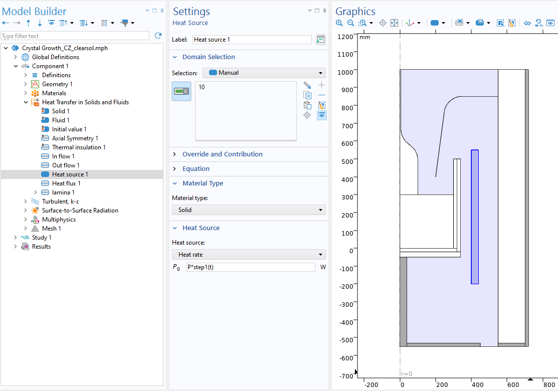
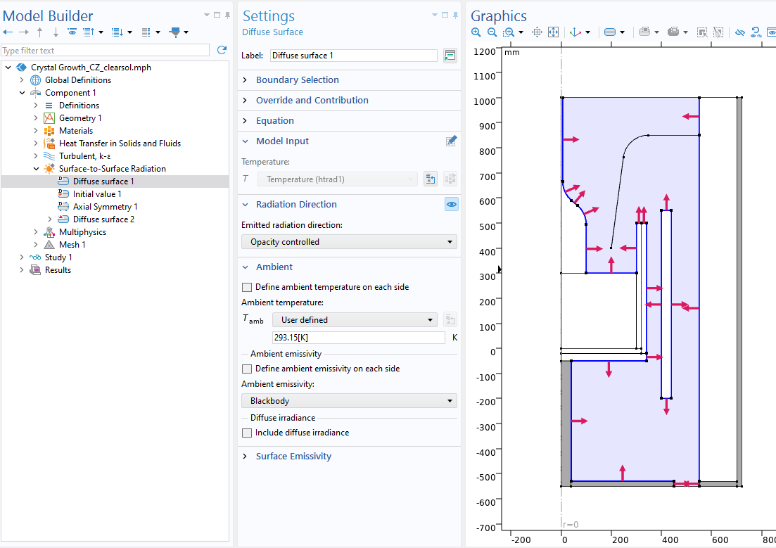
A look at the model set up in the software with heat transfer (left) and thermal radiation (right).
The tutorial Thermal Analysis of a Czochralski Crystal Growth Furnace models the process as described. The model’s geometry consists of a quartz crucible containing the melt, with the crystal rod in the middle of the melt surface, both positioned inside a furnace. Inside the furnace, a flow of argon cools the crystal rod to maintain the desired temperature gradient and to expel volatile species from the furnace. A graphite heater is placed inside the furnace to maintain a stable temperature. Both the crucible and the rod rotate at a speed of 5 rpm, but in opposite directions. The entire geometry of the described process is rotationally symmetric, enabling the use of a 2D axisymmetric model setup in COMSOL Multiphysics®.
The heat transfer in the melt, crystal rods, graphite heater, and furnace walls is modeled, assuming heat conduction as the dominant mechanism. A surface-to-surface radiation model accounts for the heat transfer between the surfaces inside the furnace. The nonisothermal flow of argon inside the furnace is modeled using a weakly compressible flow assumption with the k-ε turbulence model coupled to heat transfer in turbulent flow. Sliding wall conditions describe the rotation of the crystal rod and crucible.
Our focus is to investigate the protective gas flow and the convective heat transfer to find out the right parameters needed to maintain the required temperature gradient at the crystal growth interface.
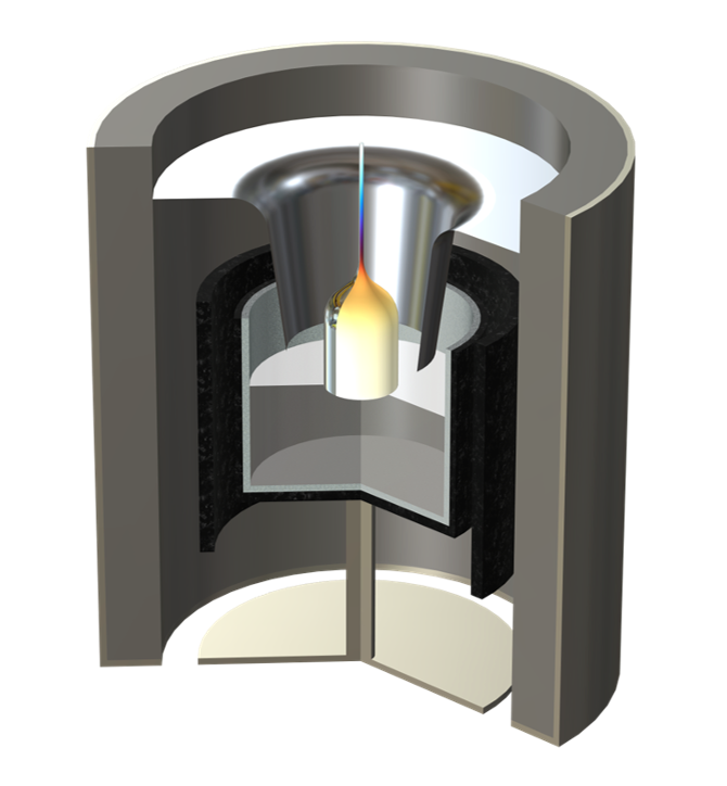 Our model crystal growth furnace.
Within the model geometry, the graphite heater operates at 310 kW and protective argon gas is introduced at a rate of 100 liters per minute. The furnace pressure is maintained at 2500 Pa. The crucible rotates at 5 rpm and the crystal rod rotates at -5 rpm, creating the necessary twisting motion for effective crystal growth. The rotational velocity of this type of furnace is much higher than pull velocity, so pull velocity was ignored in this simulation.
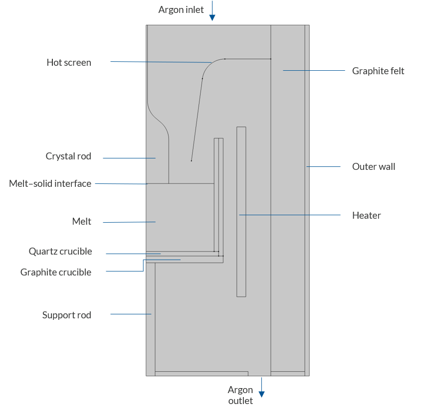 The crystal growth furnace geometry with each part labeled.
Exploring the Results
Within our model, we conducted a two-step study. The first step involves solving the flow equations at a steady state to establish good initial conditions for the subsequent time-dependent study step. In the time-dependent study step, the flow and heat transfer equations are solved fully coupled.
Flow Field
The computed flow field reveals a maximum velocity near the surface of the crystal rod. A recirculation zone exists between the hot screen and the crystal rod, driven primarily by the buoyancy from the hot screen’s high temperature and, to a lesser extent, by a slight downward flow from the inlet. This high velocity facilitates effective heat removal, resulting in a significant temperature gradient within the crystal rod.
The flow between the crucible and the heater moves downward, which is counterintuitive as one might expect a chimney effect in this area. However, this effect actually occurs outside the heater, between the heater and the furnace wall, where the flow predominantly moves upward.
It is notable that the impact of free convection in the furnace is more significant than that of the argon’s inlet and outlet flows, which are barely discernible in the plot. Without a model, predicting the entire flow field would have been challenging.
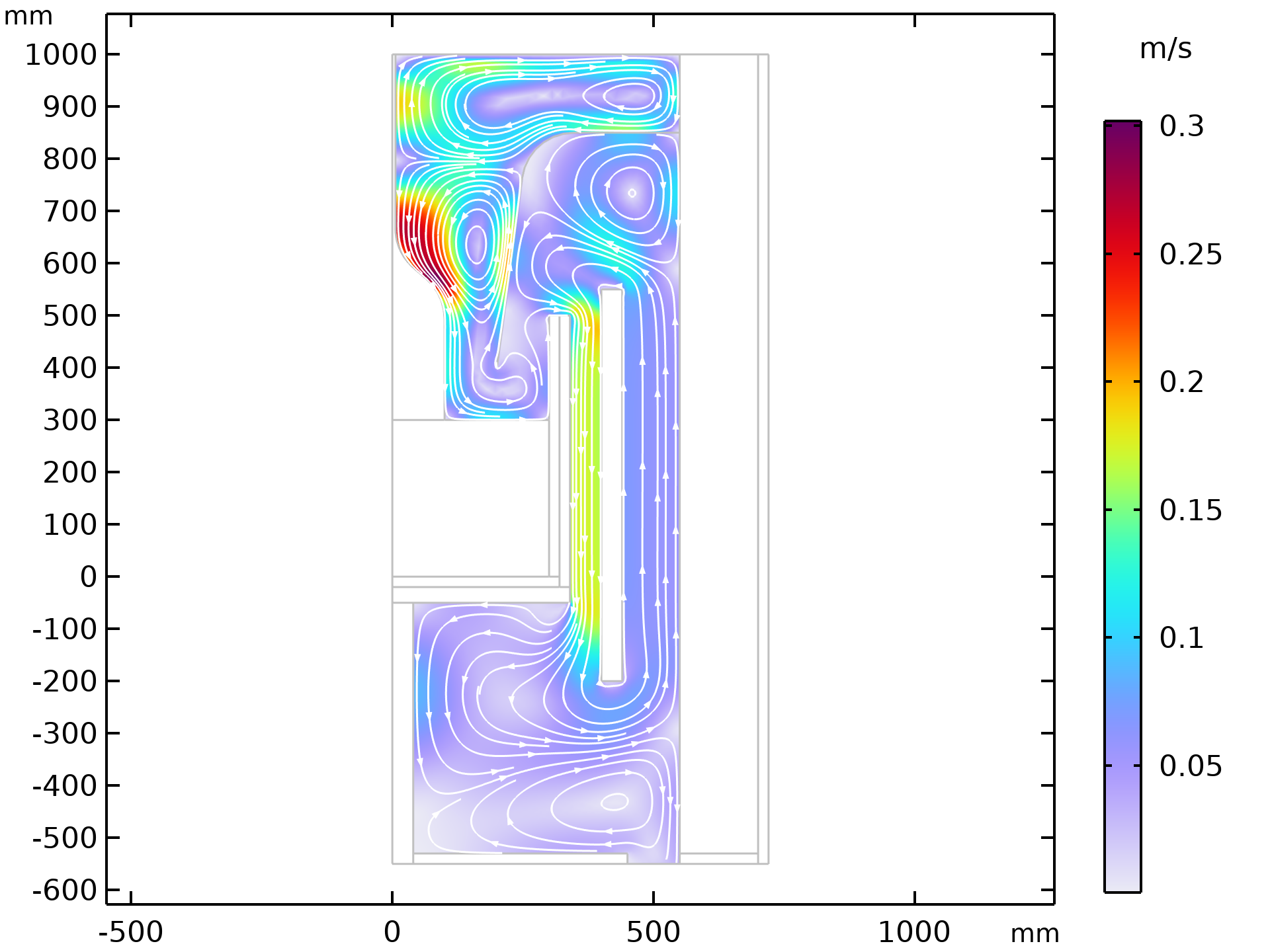 A look at the flow field within the furnace.
Temperature
Our study shows that the average temperature at the contact surface between the melt and the rod reaches a steady state after approximately 400 minutes. The melting temperature (Tm = 1414°C) contour is close to this contact surface, see the 1415°C contour curve in the plot below. The temperature at the point where the rod contacts the melt varies between 1403°C and 1407.5°C , with the highest temperature occurring in the middle of the rod. This is close to the real melting temperature of 1414°C. The temperature along the height of the rod decreases, exhibiting a gradient in the z-direction ranging from 500 to 100°C/m. This indicates that the single-crystal rod is efficiently cooled by the argon flow.
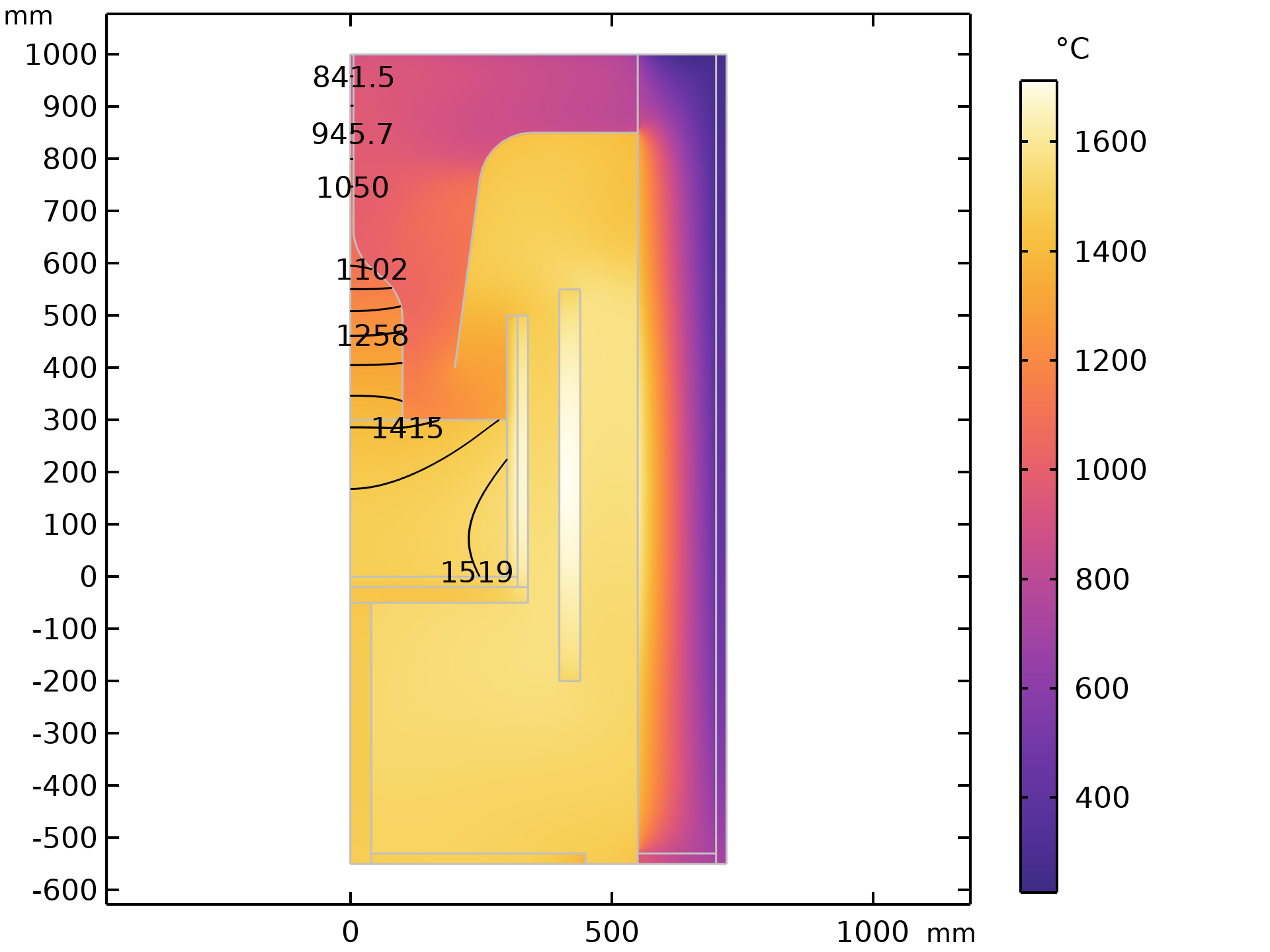
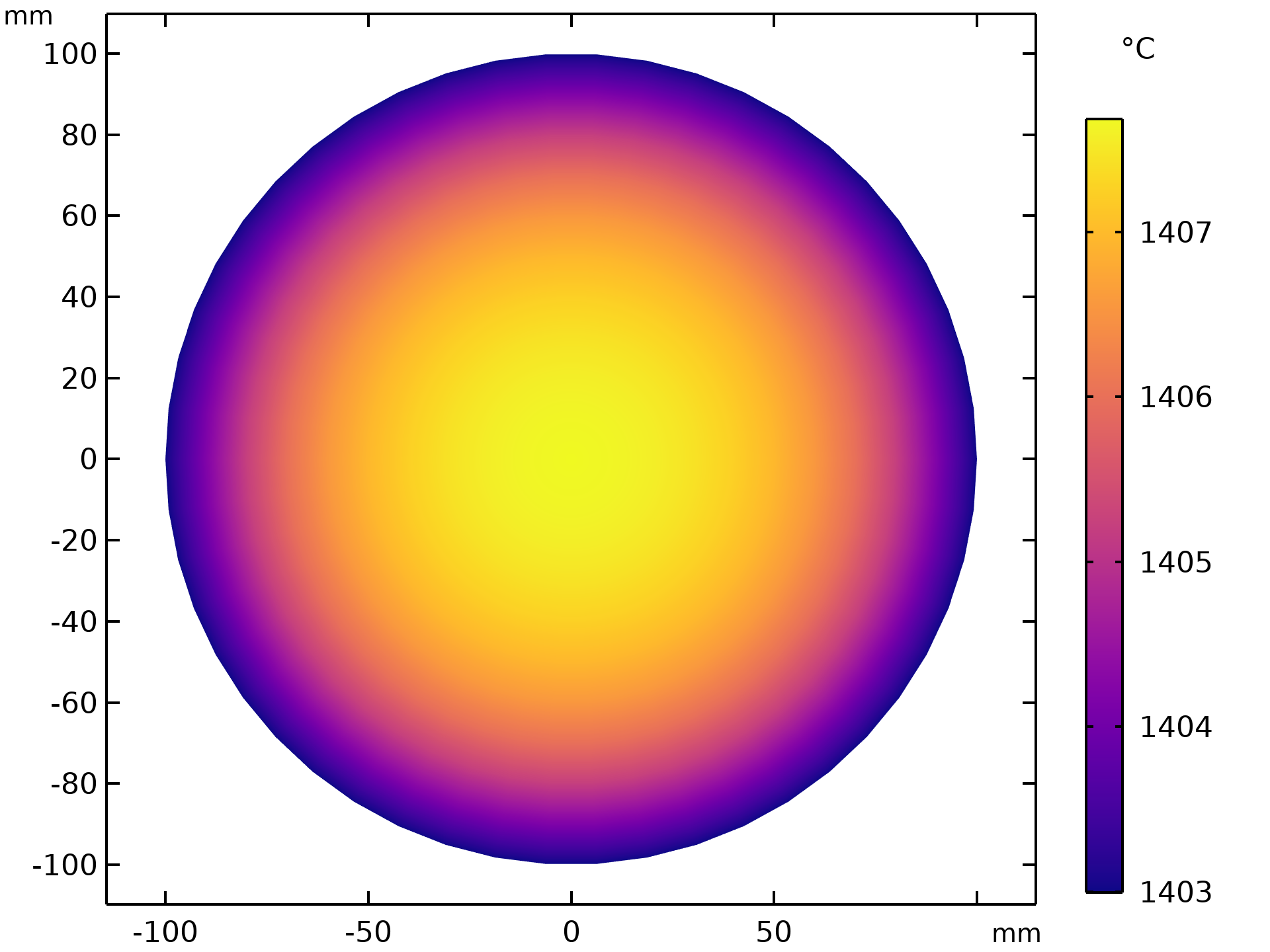
At left: Viewing the model with a focus on the average temperature at 600 minutes. At right: The temperature distribution at the surface where the rod makes contact with the melt.
Future Furnace Extensions
With this model, we treat the crystals and melts as solids and are interested in performing a thermal analysis on the design. While this model accomplishes that goal, it can be extended. For example, users could model other heating methods such as induction. A larger extension might include a focus on modeling the flow in the melt and the natural convection, surface convection (Marangoni effect), and forced convection (magnetic fluid) within it. Users can also use the Phase Change interface to see the phase change from melt to crystal as well as the solidification with latent heat and pulling of the crystal. Although the pull velocity is neglected in this demo, it could be set in the wall boundary conditions, i.e., the velocity of the tangentially moving wall.
Try it Yourself
Looking to model this Czochralski crystal growth furnace yourself? The MPH-file and step-by-step instructions are available in the Application Gallery.

Comments (0)