

Certain modeling problems can lead to particularly elegant solutions. One such case recently presented itself in the form of finding the time-periodic stationary solution to a problem involving a nonlinear electrical circuit. Let’s take a deeper look at this case and see how some of the core capabilities of the software can help provide an efficient implementation.
The Modeling Scenario: A Nonlinear Transformer
We have previously looked at the case of a transformer consisting of two coils wound around a nonlinear core material in our blog post “Using Differential Inductances and the Coil Feature”. An applied sinusoidal AC voltage will induce currents to flow in the primary and secondary coil, however, at high enough currents, the material nonlinearity will significantly alter the differential inductances, and the induced currents will be nonsinusoidal. We can model this behavior either by building a full-fidelity model of the device or by building an equivalent electrical circuit model where the nonlinear differential inductances are considered. The nonlinearities lead to currents that will be periodic, albeit nonsinusoidal in time. We can observe this gradual response by running a transient model for many periods.
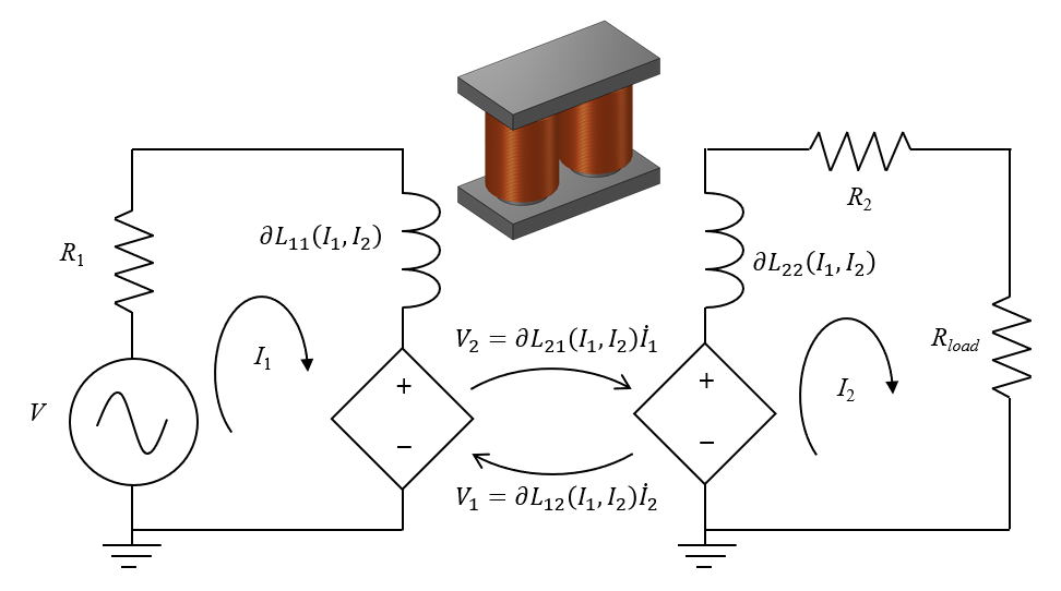
A transformer consisting of two coils wound around a nonlinear core. The differential inductances can be extracted from the finite element model and used within an equivalent circuit model.
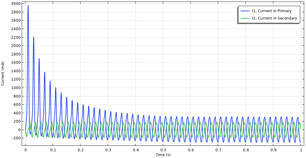
The results of running the equivalent circuit model for many periods show that the time-periodic steady state is gradually approached.
Looking at the results, it’s clear that we need to simulate for many periods, and if we are only interested in the time-periodic steady state solution, then most of the generated data is not actually needed. Ideally, in this situation, we want a method that leads directly to the time-periodic solution, and that is what we will address here.
Reformulating the Equivalent Circuit from Time to Space
If we take a closer look at our electrical circuit model, we see that it has only two time-varying unknowns: I_1 and I_2, the current through the primary and secondary. Let’s shift from looking at the circuit diagram, to now looking at this in terms of the potential drops across each element of the two current loops
where all of the differential inductances are functions of both currents: \partial L_{ij} (I_1,I_2). This set of coupled ordinary differential equations can be solved in a myriad of ways. We will restrict ourselves to the case where the applied voltage V_{AC} and the solution is time-periodic over one period, T_0.
We can see right away that this is nearly a nonlinear algebraic set of equations, except for the time derivatives of the currents. But what if we replaced these with a spatial derivative? Let’s see where that leads us!
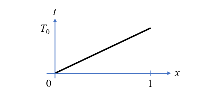
Time as a function of position along a 1D unit domain.
Consider a 1D domain — just a straight line of unit length — where we define a quasi-time variable that varies linearly along the length. If we define two spatially varying variables along this line, u_1 and u_2, and introduce a mesh along this line, then the COMSOL Multiphysics® software can take the spatial derivative, \partial u_1 / \partial x, via the differentiation operator: d(u1,x). But since we are thinking of the spatial dimension as the time dimension, this is actually the time derivative. With this in mind, we can now construct a field algebraic equation with the Domain ODEs and DAEs interface, defined over a line of unit length. The interface is shown below, where our two unknowns are defined. We will use Lagrange elements for these fields, as this automatically ensures a continuous field, and we can set the units of the fields and source appropriately. For readability, we can also define a set of variables that describe the voltage drop due to every component of the circuit model, as shown in the screenshots below.
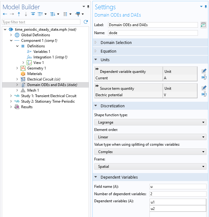
Setting up a Domain ODEs and DAEs interface, the field variables are named, the shape function is selected, and the units are set.
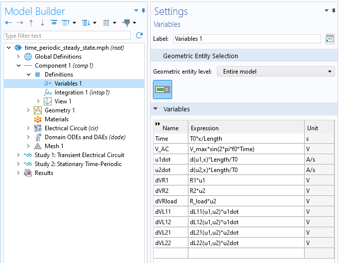
The variables that define the applied voltage in the time-space domain, the derivatives of the currents, and the voltage drops across the various components of the circuit.
These variables are used within the Algebraic Equation feature of the Domain ODEs and DAEs interface, which has two fields for an equation that must always be equal to zero. Here, we enter the sum of the potential drops, as well as the source, for the two current loops. These are the equations shown earlier. Finally, two Pointwise Constraints are added to the point at one end of the domain. The constraint here is based on an Integration feature, defined on the other point. The constraint of u1-intop1(u1) and u2-intop1(u2) enforces the periodicity condition.
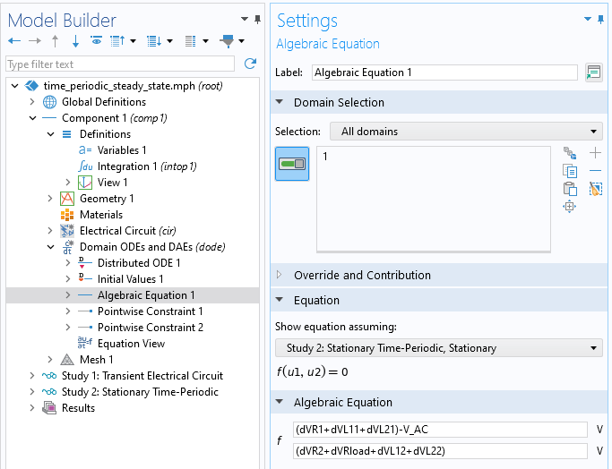
Setting up the equation that is satisfied everywhere in time-space along the unit domain.
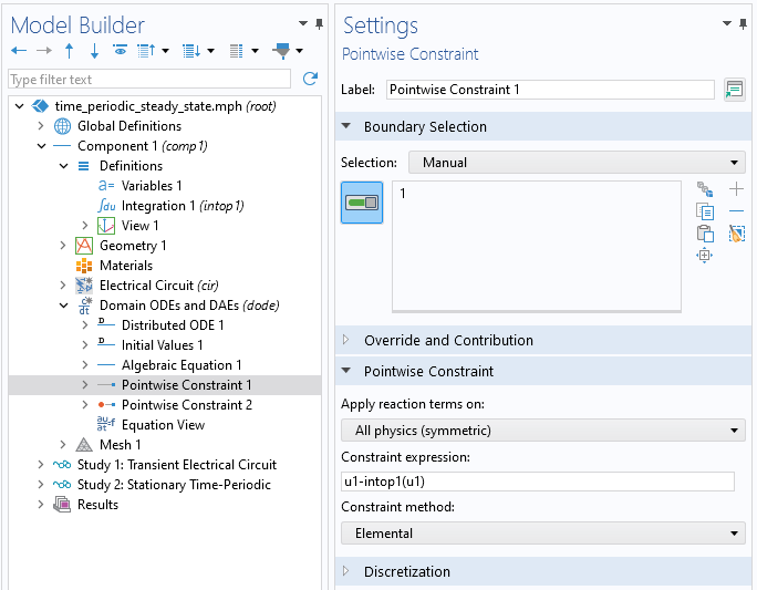
Defining the periodic condition via a Pointwise Constraint and an Integration feature.
Solving this stationary problem does require a relatively fine mesh along the domain when the device is driven into the more nonlinear regime. Thus, the mesh size along the unit line is the one parameter that needs to be studied when solving this nonlinear stationary model. The results are plotted below and compared to the transient results, showing excellent agreement. In fact, the small discrepancy can be reduced as the transient model is solved with even tighter tolerances, which will make the computational cost of even such a small model rise up a minute or so of wall-clock time, whereas the stationary problem solves nearly instantaneously.
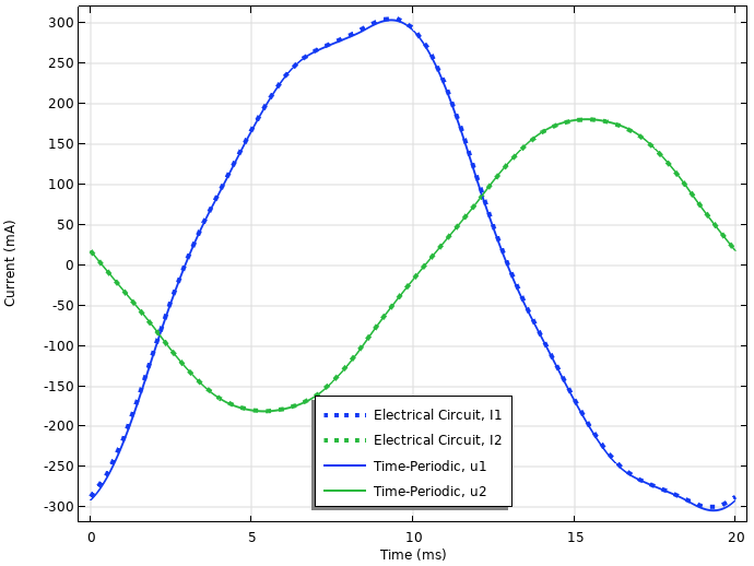
Comparison of the transient results computed from the electrical circuit model with the stationary results from the time-periodic approach.
The solution over one period in space also gives us the ability to extract the frequency content via the Spatial FFT dataset. The settings for this feature are shown in the screenshot below, highlighting an Array 1D dataset, which periodically patterns the time-space solution such that the results appear more smooth. By plotting an appropriately normalized quantity, we can see how the frequency content increases as the applied voltage is increased.
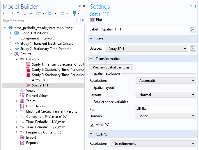
The Spatial FFT dataset takes as input the Array 1D dataset, which repeats the stationary results along the time direction.
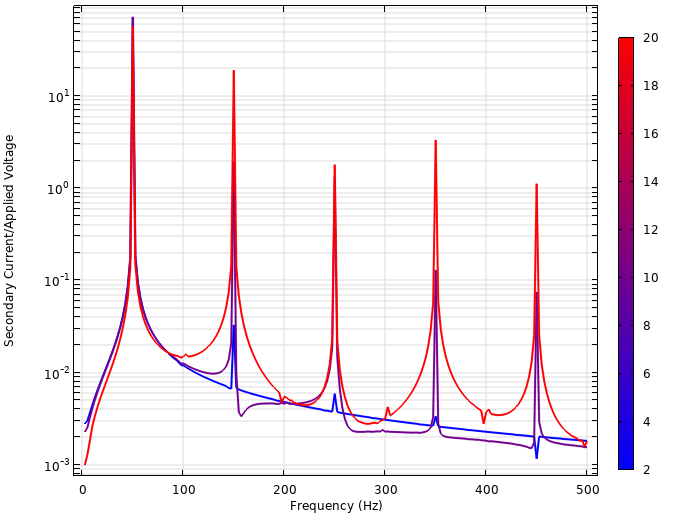
Plot of frequency content as AC voltage is increased.
Closing Remarks
In this blog post, we have looked at a particularly attractive approach if you are solving for the time-periodic steady state of a system that can be described by a set of algebraic equations. Note that this approach admits any type of applied signal — not just sinusoidal forcing functions — as long as there exists a smooth and time-periodic solution. Its setup is quite simple and takes advantage of the core functionality of COMSOL Multiphysics®, making this approach useful to any type of problem, not just electrical circuits. It is a good technique for COMSOL modelers to have in their toolbelt.
The example model related to this is available for download here:


Comments (0)