

In engineering and other sciences, a common question is what would be the effect if you combine two or more independent sources. This is often represented in graphic form as an interaction curve. In this blog post, we show some examples of interaction curves and discuss their background.
Table of Contents
- Bending and Tension of a Beam
- Power Law
- Fasteners
- Tresca Yield Criterion
- Beam Column, Revisited
- Decohesion
- Fatigue
- Safety Factors
- Isobolograms
- Final Remarks
Bending and Tension of a Beam
As an introductory example, let’s study the collapse load of a beam subjected to both an axial force and a bending moment. Assume an elastoplastic material like steel, which has identical properties in tension and compression, and a beam with a rectangular cross section of height 2a and width 2b. Ideal plasticity with a yield stress \sigma_{\mathrm y} is used as the failure criterion.
At collapse, the stress is equal to the yield stress over the whole cross section, either in tension or compression. The stress distribution can be visualized as shown below:
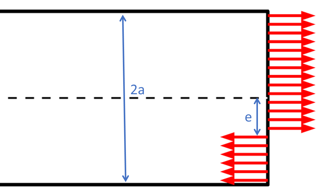 Stress distribution in a failure state.
Here, e is the distance from the center axis to the location of the stress reversal (the neutral line).
Equilibrium between the stress distribution on one side, and the applied axial force N and bending moment M on the other side, gives
and
It can immediately be seen that the maximum load-carrying capacities, N_{\mathrm f} and \displaystyle M_{\mathrm f}, are obtained when e = a and e = 0, respectively:
and
where A is the cross-section area, and Zp is the so-called “plastic section modulus”.
Often, these types of expressions are written on a nondimensional form:
and
In this case, it is easy to eliminate the parameter e so that an explicit relation can be obtained:
or equally
This expression provides the combinations of force and moment that cause failure of the beam section. A relation like this is often presented in the form of an interaction curve. The equation or corresponding graph can be used for quick evaluation of allowable states.
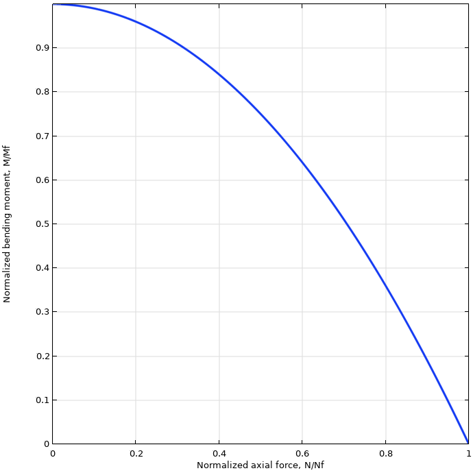 Interaction curve for a rectangular steel beam.
For nondimensional interaction laws, the most common form is to express the failure curve as f( \xi, \eta ) = 1, so that f( \xi, \eta ) < 1 represents the safe region. For the beam bending example, \eta + \xi^2 = 1.
Power Law
Many interaction rules are of a power law type. Mathematically, this means that
The exponents \alpha and \beta are not necessarily integers, even though values of one and two are common. Often, \alpha = \beta. When this is the case, the rule is symmetric in the two parameters. However, this is not always the case; the initial beam example, for instance, shows a case where \alpha \neq \beta.
With a power law, the maximum value for one parameter always occurs when the other one is zero. This seems intuitively obvious, but a counterexample will be given later on.
One special case of a power law is \alpha = \beta = 1, which results in an interaction that is purely additive and would be represented by a straight line. If you apply 40% of the critical value for one load, you can apply 60% of the other.
Fasteners
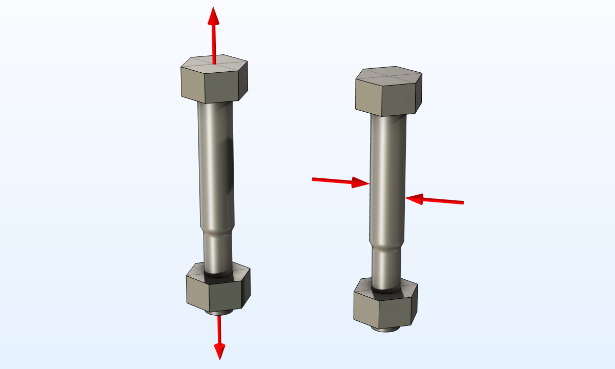
An example of a power law with \alpha = \beta = 2 is obtained by a straightforward analysis of rivets. Rivets can be subjected to a combination of tensile forces (N) and shear forces (T). The tensile stress in the rivet is
where A is the cross-section area. In an elastic state, the shear stress has a complicated distribution over the cross section, but since here we are mainly concerned with the failure state, it can be assumed that the shear stress is evenly distributed so that
Using a von Mises equivalent stress, the failure criterion is
Squaring both sides and dividing by the yield stress, the failure relation can be written as
The individual failure loads are
and
The failure load in shear is an effect of the assumed von Mises criterion.
The final result in terms of forces is then
This is an example of a power law with \alpha = \beta = 2. Such laws are common when norms of the type “square root of sum of squares” are used to combine the different effects.
However, this is not the whole truth about all types of fasteners. In older versions of MIL-HDBK-5H, Military Handbook: Metallic Materials and Elements for Aerospace Vehicle Structures (Ref. 1), several interaction rules have been suggested for bolts. Bolts are not identical to rivets, but under the conservative assumption that friction between the joined parts is ignored, the situation is similar. Using the notation from that document (t = tension; s = shear),
and
Interestingly enough, all the following interaction rules are reported:
The corresponding interaction curves are shown in the figure below.
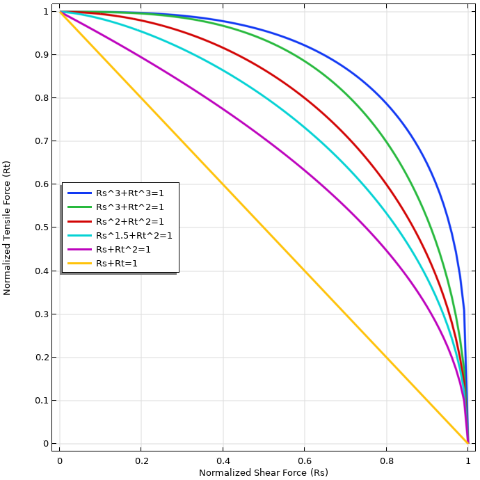 Interaction curves for different bolt interaction rules. The red curve is the one given by rivet theory.
Currently, the preferred version of the interaction rule for bolts is
How can this difference from the rivet analysis (where both terms have the exponent 2) be explained?
The suggested rule allows higher loading than what the analysis of the rivets indicates. Without having access to the underlying reasoning, it is only possible to make a guess. One important difference is that the forces for the bolts are not normalized by the failure stress, but with an “allowed force”. The allowed force in bolts is based on two different areas: The allowed tensile force is based on the threaded region, and the allowed shear force is based on the shank. It is, to some extent, two different mechanisms that govern the failure. The cross-section area in the threaded region is significantly smaller, by maybe 25%.
Taking this into account, there are actually two competing criteria:
- Failure caused by tensile overloading of the threaded area
- Failure caused by combined tensile and shear loading in the shank area
 Under pure tension, the thread will be the weakest part. Under pure shear, it is the shank. Under a combined loading, either location can be critical.
In the shank, a von Mises criterion can be used. There, the bolt (under conservative assumptions) acts like a rivet.
Here, \kappa is the ratio between the cross-section areas of the shank and the thread. This accounts for the fact that N_{\mathrm f } is defined with respect to the threaded region, and the tensile failure load in the shank is higher.
In the thread, which is not subjected to any shear, the failure criterion is simple:
Using \kappa = 1.25, the criteria can be visualized as:
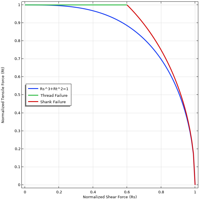 Comparison of the suggested interaction curve (blue), and a composition of shank and thread failure.
As can be seen, the von Mises based rule and the R_{\mathrm s}^3 + R_{\mathrm t}^2 = 1 rule coincide well for cases dominated by shear. For all ratios between pure tension and pure shear, the latter rule is on the conservative side. Using a single simple analytical curve makes life easier than using the piecewise function (which would be unique to every bolt size since the area ratio κ differs).
Below, a screenshot from the Safety subnode under Fasteners in the Shell interface in the COMSOL Multiphysics® software is shown. Any type of power law can be used.
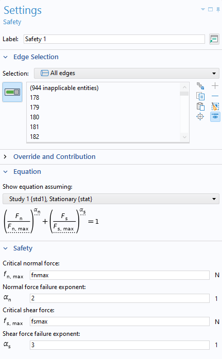 Settings for computing safety factors for fasteners in COMSOL Multiphysics®.
Tresca Yield Criterion
Previously, it was noted that using a von Mises yield stress leads to a power law with
A natural question is then: If a Tresca failure criterion is used, how does that affect the interaction curve? In standards, it is often the more conservative (but mathematically less palatable) Tresca criterion that is used.
The Tresca equivalent stress is defined as the difference between the largest and smallest principal stress. We can then resort to Mohr’s circle to perform the analysis. For a stress state that consists of a single direct stress and a shear stress, the diameter of Mohr’s circle (2R) is also the difference between the two principal stresses. Thus, the circle describing failure is
According to the Tresca criterion, the failure stress in pure shear is
The amazing result is that we retrieve exactly the same power law interaction curve as for the von Mises criterion!
The only difference is that the failure load for shear used in the expression, {T_{\mathrm f}} , is 13% smaller when the Tresca criterion is used.
Beam Column, Revisited
Beam columns are often made from concrete. Concrete is a material for which the strength in compression differs significantly from the strength in tension. The tensile strength, \sigma_{\mathrm t}, is only of the order of 10% of the compressive strength, \sigma_{\mathrm c}.
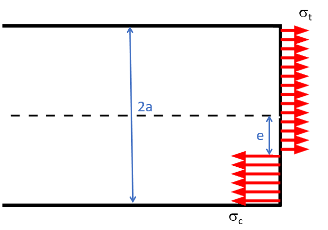 Stress distribution in a failure state when the compressive stress is higher than the tensile stress.
If the initial analysis of a rectangular beam is repeated, taking the different tensile and compressive stresses into account, we get
and
Before continuing, an important remark must be made: In practice, concrete is always reinforced, usually with steel bars. A full analysis requires that the amount of reinforcement, its placement in the cross section, and its yield stress are taken into account. All of this complicates the algebra significantly. The current simplified analysis still serves the purpose to show the principles.
As reference failure load for axial force, we can choose the failure in pure compression, that is
As failure load for bending, the maximum possible moment is chosen. It is evident that it occurs when e = 0, so that
Let’s introduce a parameter \beta for the ratio between tensile strength and compressive strength, such that \sigma_{\mathrm t } = \beta \sigma_{\mathrm c }. Also, let e = \epsilon a. This will make it easier to write nondimensional relations. Now,
and
Here, the compressive load is taken as positive (P = -N). This is a customary convention for columns, since the intended loading is predominantly in compression.
The interaction curve is shown below for \beta = 0.1, using the convention that the force is plotted on the vertical axis and the bending moment is plotted on the horizontal axis.
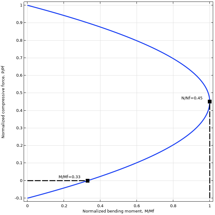 Interaction curve for a concrete beam.
Note that, in this case, the maximum allowable moment does not coincide with zero axial force. As can be seen from the above expressions, the maximum moment capacity occurs when
Since \beta is small, the maximum moment capacity, somewhat surprisingly, occurs when the compressive force is almost 50% of the failure load. From the graph, it is also possible to infer that when there is no axial force, the moment capacity is reduced by 70% from its maximum value!
If the reinforcement is taken into account, the shape of the interaction curve changes, but not in a fundamental way. To see such diagrams, you can perform a web search for “column interaction curve”.
Decohesion
Decohesion between two bonded surfaces is usually considered a combination of failure in tension and failure in shear. The load-carrying capacity is, in this case, usually described by the fracture toughness for mode I (tension) and mode II (shear), G_{\mathrm {Ic}} and G_{\mathrm {IIc}}.
One of the earliest suggested interaction rules for describing mixed-mode decohesion was a power law,
In this case, the exponents \alpha and \beta must be matched to experiments. There is no first principle on which to rely. You can view this model as having either two parameters (\alpha and \beta) with the values of G_{\mathrm {Ic}} and G_{\mathrm {IIc}} determined from single-mode experiments. Alternatively, all four parameters can be used to get the best possible match to a set of experiments with different mode mixtures. In that case, G_{\mathrm {Ic}} and G_{\mathrm {IIc}} will not exactly match the result of pure tensile or shear tests.
In many cases, the power law does not match measurements well enough. Another popular interaction law is provided by the Benzeggagh–Kenane (B-K) criterion:
The interpretation of this rule is not obvious. It states that the sum of the applied mode I and mode II energy release rates equals an effective fracture toughness G_{\mathrm {c}} at failure:
The effective fracture toughness is a weighted sum of G_{\mathrm {Ic}} and G_{\mathrm {IIc}}, where the weighting depends on the ratio between the applied loads. It is easily seen that for pure mode I, or pure mode II, the single-mode criteria are recovered. In order to understand the implications of the B-K criterion, an interaction curve can be elucidating.
If the unidirectional strengths have been measured, there is only one parameter that must be matched to experiments, the exponent \eta. Alternatively, all three parameters can be used for better curve fitting.
The interaction curve can be parametrized using a parameter describing the loading,
R will vary from 0 (pure mode I) to 1 (pure mode II).
Let the ratio between the shear and tensile fracture toughness be \kappa so that
Usually, \kappa < 1.
By some reordering, the B-K criterion can then be written on a nondimensional form as either
or
This can be viewed as a parametric description of the interaction curve, with R as the parameter.
In the table below, material parameters for four different materials are given for both the B-K criterion and the power law. The data is taken from Ref. 2. The values for the fracture toughness, G_{\mathrm {Ic}} and G_{\mathrm {IIc}}, are not the same for both models. The fracture toughness values have been part of the overall curve fitting.
| Material | \kappa | \eta | \alpha | \beta |
|---|---|---|---|---|
| 1 | 0.147 | 1.75 | 0.17 | 4.8 |
| 2 | 0.0785 | 2.35 | 6.0 | 6.0 |
| 3 | 0.0182 | 1.39 | 0.49 | 3.9 |
| 4 | 0.783 | 0.63 | 2.1 | 0.62 |
This data is plotted as interaction curves below. The curves for the power law have been scaled with respect to the difference in fracture toughness between the models. This is why the graphs for the power law do not end at a value of 1.
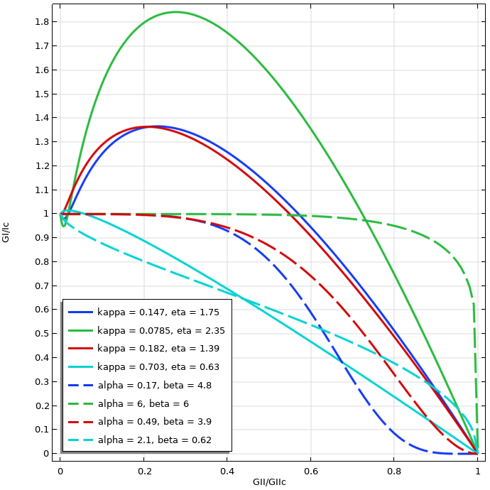 Interaction curves for mixed-mode decohesion for four different materials. Solid lines show the B-K criterion, and dashed lines show the power law criterion for the same material.
As can be seen, the interaction curves have some surprising properties, which are effects of their individual mathematical properties. When presented this way, it is clear the predictions for the same material may differ significantly depending on the model used.
An example where the B-K criterion is used for modeling decohesion can be found in the Mixed-Mode Debonding of a Laminated Composite tutorial model.
Fatigue
When evaluating the risk of fatigue failure, it is usually recognized that the allowed stress amplitude depends on the mean stress. A high tensile mean stress reduces the allowed stress variation. Several rules are in use, leading to different interaction curves between mean stress and stress amplitude. Three of the most common rules are called Goodman, Gerber, and Soderberg.
If the allowed amplitude stress is called \sigma_{\mathrm a} and the mean stress is called \sigma_{\mathrm m}, then these rules state:
Goodman:
Gerber:
Soderberg:
The allowed stress amplitude has been normalized by the fatigue limit at zero mean stress, \sigma_{\mathrm a0}. \sigma_{\mathrm u} and \sigma_{\mathrm y } denote the ultimate stress and yield stress, respectively. These rules can be visualized as interaction curves.
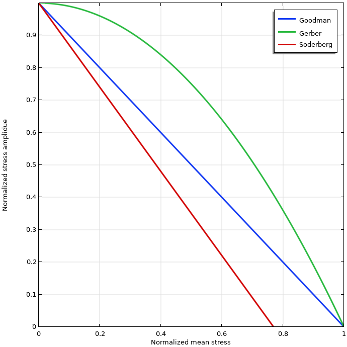 Interaction between stress amplitude and mean stress for fatigue evaluation. The mean stress axis is normalized by the ultimate stress, and the ultimate stress is assumed to be 30% larger than the yield stress.
Safety Factors
When you have a failure criterion, a common requirement is to present a single safety factor, margin of safety, or similar quantity. This is, of course, reasonable, but it is not always trivial. In most cases, you expect a safety factor to represent how much you can scale the load until you reach failure. However, the whole idea of interaction curves is that there are two independent sources. Using the notation that failure is represented by f( \xi, \eta ) = 1, let’s consider a safe state f( \xi_0, \eta_0) = q < 1. There are at least three reasonable definitions of a safety factor, s:
- Safety factor against increasing the first load, keeping the second load fixed: f( s\xi_0, \eta_0) = 1
- Safety factor against increasing the second load, keeping the first load fixed: f( \xi_0, s\eta_0) = 1
- Safety factor against a proportional increase of the two loads: f( s\xi_0, s\eta_0) = 1
In most cases, computing the safety factor according to any of these three relations requires the solution of a nonlinear equation.
As an example, assume the beam in the initial example is loaded to a level where
In the figure below, the three interpretations of safety factors are illustrated graphically. The interaction curve can easily be used for graphically finding safety factors without solving equations.
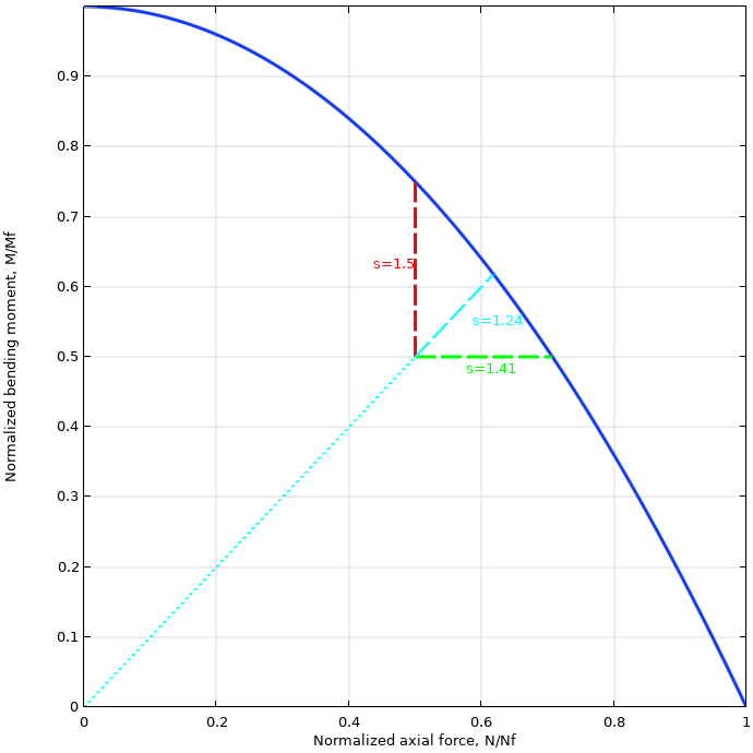 Interaction curve, together with three different types of safety factors.
In this case, the three equations for the safety factor give
Isobolograms
Let’s now look at the use of interaction curves outside of the realm of structural mechanics. Isobolograms are used to determine the interaction between drug products for medical use.
Two drugs administered at the same time can enhance the effect of each other. This is called “synergy”. However, it is also quite possible that they will counteract each other, termed “antagonism”. Synergistic effects can be desirable since they can lead to reduced doses, which in turn could result in less side effects.
The same ideas can, of course, also be applied to toxicity, when mixing two toxic substances can give an effect that is either stronger or weaker than the sum of the two individual effects.
An isobologram is an interaction curve between two substances, showing the combinations that lead to the same effect. As usual, the curve is normalized. In the figure below, the principal shapes of isobolograms are shown.
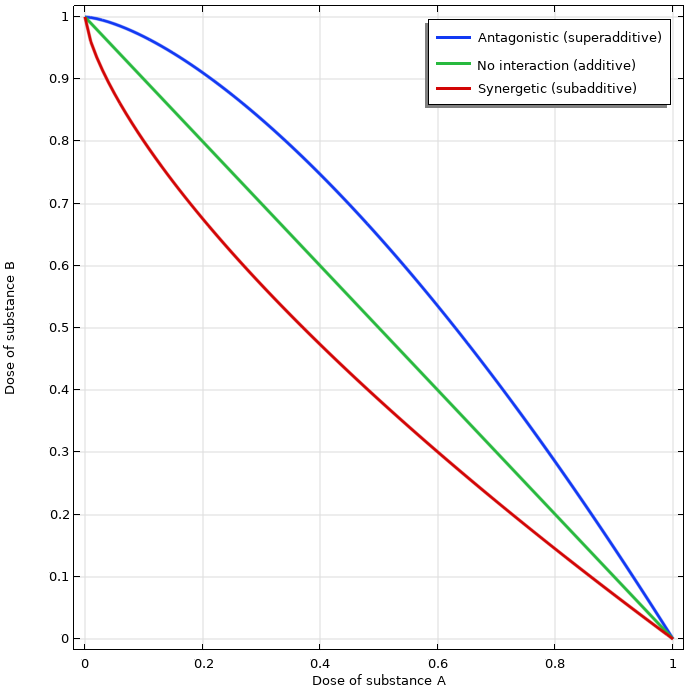 Isobolograms for three different types of drug interactions.
Final Remarks
Interaction diagrams are powerful tools for understanding the combined effect of two actions, both from a qualitative and a quantitative perspective.
It seems like most structural failure curves are of the antagonistic kind, and it is usually possible to sustain two different loads better than what a pure addition would suggest. But is that always true? I cannot answer that question, but if you have some nice counterexamples, please add your comments. As a matter of fact, some of the earlier graphs for decohesion do exhibit synergetic behavior in part of the range. This may, however, be an artifact that comes from the curve fitting. Any power law with an exponent <1 will partially fall below the additive line.
References
- MIL-HDBK-5H, Military Handbook: Metallic Materials and Elements for Aerospace Vehicle Structures, 1998; http://everyspec.com/MIL-HDBK/MIL-HDBK-0001-0099/MIL_HDBK_5H_1804/
- J.R. Reeder, “3-D Mixed Mode Delamination Fracture Criteria – An Experimentalist’s Perspective,” NASA Langley Research Center, 2006; https://ntrs.nasa.gov/citations/20060048260


Comments (1)
Jay Puckett
February 15, 2025Henrik
Thank you, well done.
I found this Comsol blog particularly interesting because it covers many important topics in a short, well-written piece. Over the years, I have used most of these (and several are embedded in the specifications). The safety factor is especially important for load rating for interactions, something that the AASHTO community only in recent years has successfully discussed and documented in examples (MCFT=shear-moment interaction for concrete). (or eliminated in the spirit of simplification V-M steel).
As a structural engineer, expanding this to reinforced concrete axial-moment interaction would be great.
Jay