How to Postprocess Fields over Arbitrary Geometries

Have you ever wanted to query the results of your model within an arbitrary geometric subregion? You might think that this requires adding geometries to a model and recomputing the solution. Instead, in the COMSOL Multiphysics® software, we can just add and reposition a part solely for the purpose of evaluating the results. We will demonstrate this in the context of computing mutual inductance between coils and discuss simpler techniques that can be used for a reduced set of cases.

Computing Mutual Inductance

Let’s consider the model shown below of two current-carrying circular coils, each carrying a current of I₀ = 0.25 mA. The magnetic flux density, the B-field, is plotted in the space around these primary coils. Suppose that we want to introduce a smaller pickup coil in the space between the larger primary coils. This pickup coil intercepts part of the magnetic flux and is defined by its outside perimeter curve C and enclosed area A.

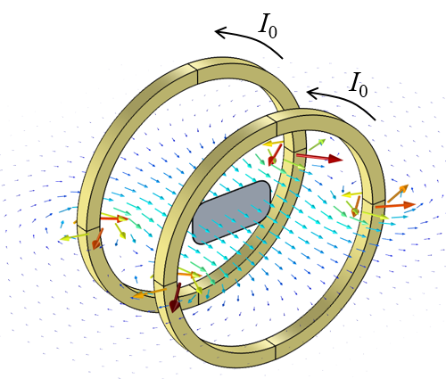
The magnetic flux density around a Helmholtz coil with a pickup coil inside. The enclosed area of the coil is shaded in gray. We want to recompute the mutual inductance as the pickup coil changes orientation.

The mutual inductance between these primary and pickup coils is defined as:

where n is a vector normal to the surface A.

Since the B-field is computed from the magnetic vector potential, \mathbf{B=\nabla \times A}, we can use Stokes’ theorem to see that the above surface integral is equivalent to the line integral:

where t is the tangent vector to the curve C.

This method of computing mutual inductance is also shown in the Application Gallery example of an RFID system.

We can place the pickup coil at any location and orientation around the primary coils, solve the model, and evaluate either of the above integrals. We can even add the pickup coil geometry features after solving the model by using the Update Solution functionality. This functionality remeshes the entire model geometry and maps the previously computed solution from the old mesh onto the new mesh. This is appropriate and easy to do if the changes to the geometry do not affect the solution and if we only want to try out a few different pickup coil locations.

Suppose that we want to try out many different locations and orientations for the pickup coil. Since the A-field doesn’t change, we don’t want to re-solve or remesh the entire model, but just want to move the pickup coil geometry around. We can achieve this by using a combination of multiple geometry components, the General Extrusion component coupling, and Integration component couplings.

Implementing an Integration over Arbitrary Geometries in COMSOL Multiphysics®

We begin with the existing Helmholtz coil example and introduce another 3D component into our model. The geometry within this second component is used to define the pickup coil’s edges, cross-sectional surface, and orientation. The Rotate and Move geometry features enable us to reorient the coil into any position that we would like. For visualization purposes, we can also include the edges that define the primary coils, as shown in the screenshot below.

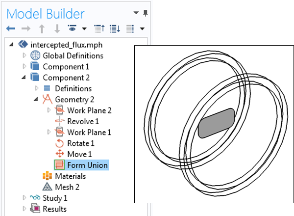
The setup of a second component and geometry.

The spatial coordinates of Component 2 overlap exactly with Component 1, but otherwise there is no connection between the two. A mapping is introduced via the General Extrusion component coupling that is defined in Component 1. This coupling uses a Source Selection for all of the domains in Component 1. Whenever this coupling is evaluated at a point in space in Component 2, it takes the fields at the same point in space in Component 1.

The approach of using two components and mapping the solution between them is also introduced in the Submodeling Analysis of a Shaft tutorial model.

Within Component 2, we define two Integration component couplings, one defined over the edges of the pickup coil, named intC, and the other over the cross-sectional boundary, named intA. This allows us to compute the mutual inductance with either of the above approaches by defining two variables. These variables, named L_C and L_A, are defined via the equations:

intC(t1x*comp1.genext1(comp1.Ax)+t1y*comp1.genext1(comp1.Ay)+t1z*comp1.genext1(comp1.Az))/I0

and

intA(nx*comp1.genext1(comp1.mf.Bx)+ny*comp1.genext1(comp1.mf.By)+nz*comp1.genext1(comp1.mf.Bz))/I0

Here, t1, t1y, and t1z are the components of the tangent vector to the pickup coil perimeter; nx, ny, and nz are the components of the normal vector to the pickup coil surface; and I₀ = 0.25 mA is a global parameter.

Since there are multiple components in the model, we must use the full name of the component couplings and fields that reside within Component 1. Also, note that the normal vector and perimeter tangent vector can be oriented in one of two opposite directions, which results in a sign change that we need to be aware of.

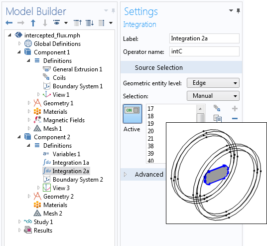
Integration component coupling defined over the pickup coil perimeter in the second component.

We can also sweep over different positions and orientations of the pickup coil. We already have the solution for the magnetic fields computed in Study 1. We add a second study that includes a parametric sweep, but does not solve for any physics. Within the study step settings, we can specify that we want to use the existing solution for the magnetic field, as shown in the screenshot below.

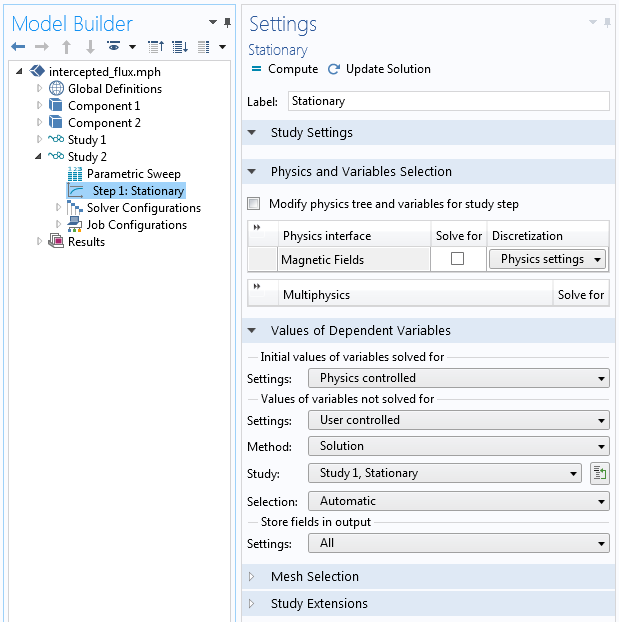
Study step settings showing how the solution from Study 1 is used in Study 2.

This second study takes relatively little computational resources when compared to remeshing the entire model and re-solving for the magnetic fields. For each different position of the pickup coil, the software only needs to remesh the pickup coil surface. The solution from Study 1 is then mapped onto this new pickup coil position and the two variables are evaluated.

This approach also works for nonplanar integration surfaces and multiturn integration curves, as demonstrated in the RFID example. Not only can the integration edges and surfaces be almost arbitrary, but they can also easily be reoriented into any position using the Rotate and Move geometry operations. Thus, this is a very general approach for evaluating fields over arbitrary geometries and locations.

A Simpler Approach: Using Cut Planes

Now that we’ve seen the most flexible approach, which enables us to perform an integration over an arbitrary shape, let’s look at a simpler case. Suppose that we are dealing with a planar integration surface and the surface edges can easily be defined in terms of the x– and y-coordinates relative to an origin point on that plane.

The first step in this approach is to take a slice (cut plane) through the entire modeling space. We can do this via the Cut Plane data set, as described in this blog post on computing the total normal flux on a planar surface. We can control the origin of the cut plane and the normal vector to the cut plane via the global parameters. Also, note that the cut plane defines local variables called cpl1x and cpl1y for the local x and y locations, respectively, as well as cpl1nx, cpl1ny, and cpl1nz for the components of the normal vector to the plane.

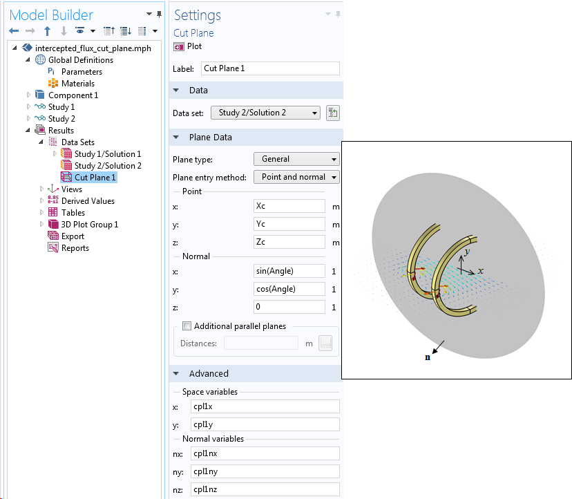
Using the Cut Plane data set. The origin point and normal are defined in terms of global parameters. The advanced settings show the names of the local x– and y-coordinates and normal coordinates.

We can now perform a surface integration over this entire cut plane, but we want to restrict ourselves to a subspace within this plane. We do this by using a space-dependent logical expression that evaluates to true (or 1) within our area of interest and false (or 0) elsewhere. This logical expression multiplies our integrand. In the screenshot below, for example, we see the surface integration performed over the cut plane is the expression:

-(sqrt(cpl1x^2+cpl1y^2)<0.1[m])*(cpl1nx*mf.Bx+cpl1ny*mf.By+cpl1nz*mf.Bz)/I0

which includes the logical expression (sqrt(cpl1x^2+cpl1y^2)<0.1[m]) that evaluates to 1 within a circle with a 0.1-m radius centered at the origin.

The remainder of the expression evaluates the flux dotted with the cut plane normal vector, thus giving us the flux through a 0.1-m-radius circle centered at the cut plane origin.

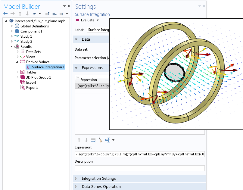
The evaluation of an integral over a subregion of a cut plane using logical expressions.

The boundaries of the subregion within the cut plane are a bit jagged; however, this gets reduced with mesh refinement. As in the earlier approach, we use a second study with a parametric sweep to store all of the different orientations of the cut plane in a second data set. In this case, there isn’t a second component or geometry that is getting reoriented and remeshed, so the evaluation is faster.

An Even Simpler Approach: Using Parameterized Curves

Let’s now look at an even simpler approach that is useful in a smaller set of cases. Suppose that we want to integrate along a curve that can be described via a parametric equation. One of the simplest curves to describe via a parametric equation is the unit circle on the xy-plane, which is defined by x=cos(s), y=sin(s) for 0\le s \le 2\pi. It’s also straightforward to compute the tangent vector for any parametric curve. For a unit circle, the tangent vector components are:

We can use these simple equations within a Parameterized Curve 3D data set for a 0.1-m-radius circle lying in the xz-plane. The circle’s centerpoint is offset from the global origin via a set of global parameters.

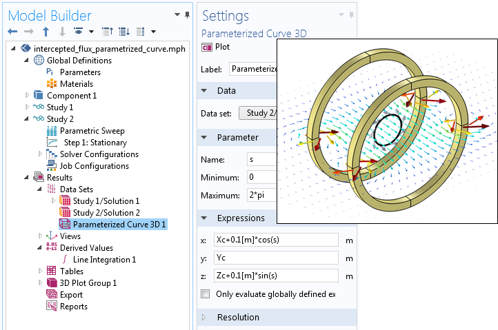
Settings in a Parametric Curve 3D data set. The curve is shown in black and the tangent vector arrows in gray.

We can create a second data set with another study and use a parametric sweep to evaluate many different origin points for the circle. We then perform a line integral over this new data set, as shown in the screenshot below. The integrand

(-sin(s)*Ax+0*Ay+cos(s)*Az)/I0

assumes a circle in the xz-plane and evaluates the A-field along the parametric curve.

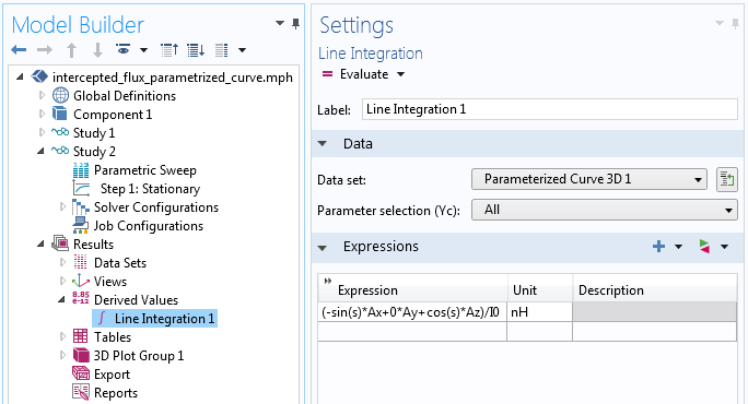
The line integration over a Parametric Curve data set.

Of the three approaches, this is the simplest and most accurate for a given mesh discretization, but also has the most limitations. Writing parametric equations for curves other than circles, ellipses, and squares aligned with the coordinate axes is more difficult.

In the figure below, we plot and compare the results for all of these approaches for a circular integration area moved back and forth along the coil axis.

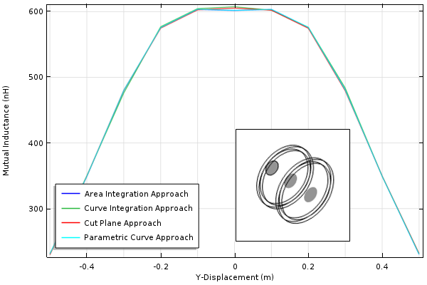
Comparison of the various approaches for computing mutual inductance.

Concluding Thoughts on Postprocessing Fields over Arbitrary Geometries

Here, we have shown three approaches for extracting surface and line integrals over subregions within a modeling space. The first approach is the most general; it allows integration over arbitrary (and even nonplanar) surfaces and curves. The first approach also allows arbitrary reorientation of the geometries being integrated over. While this approach is the most flexible, it also requires the most work to set up.

The second approach (using a Cut Plane data set) is applicable only to planar integration surfaces and is more limited in the shapes of integration surfaces that can be considered. The third approach (using a parameterized curve) is the quickest and simplest to implement, but is best suited for simple integration curves such as circles.

Further Resources

• Learn more about integration over subregions on the COMSOL Blog
  • Maximum Evaluations on Parallel Sections
  • Computing Total Normal Flux on a Planar Surface
• Find out how to use the General Extrusion component coupling in these blog posts:
  • Using the General Extrusion Coupling Operator in COMSOL: Dynamic Probe
  • Accessing Nonlocal Variables with Linear Extrusion Operators
  • Part 2: Mapping Variables with General Extrusion Operators