Learning Center

More on PCE Surrogate Models

---

This part of the course provides an introduction to the theory behind polynomial chaos expansion (PCE) surrogate models. For examples of how PCE surrogate models can be used, see the Introduction to Uncertainty Quantification course and parts of the Introduction to Surrogate Modeling course.

Introduction to PCE Surrogate Models

Polynomial Chaos Expansion (PCE) surrogate models are mainly used for uncertainty quantification, particularly for sensitivity analysis, as demonstrated in the article on Sensitivity Analysis Using a Polynomial Chaos Expansion Surrogate Model. PCE represents the uncertain parameters of a system as a series of orthogonal polynomials, chosen based on the probability distributions of the input variables. For example, Hermite polynomials are used for normal (Gaussian) distributions, while Legendre polynomials are used for uniform distributions. By projecting the output of a finite element model (or other numerical models) onto this polynomial basis, an efficient and accurate surrogate model can be constructed. Note that in a case where the parameters are not uncertain, but merely input parameters to the surrogate model, a uniform distribution is typically used.

PCE surrogate models offer a valuable alternative to Gaussian Process (GP) surrogate models, eliminating the need for hyperparameter optimization or selecting a covariance function. Instead, PCE requires selecting a predefined probability distribution for each input parameter, which determines the type of orthogonal polynomial basis. The degree of approximation in PCE is easily adjustable by truncating the polynomial expansion to the desired polynomial degree, allowing for the creation of a more approximate model when necessary, such as for an initial sensitivity analysis. A PCE surrogate model provides a direct method for computing Sobol indices used in global sensitivity analysis. For more detailed analyses, such as uncertainty propagation or localized standard deviation estimates, a GP model can be used in subsequent steps.

Polynomial Chaos Expansion in One Variable

When performing PCE regression, we assume that the uncertainty in the model inputs can be represented by a set of orthogonal polynomials. The PCE approach transforms the original uncertain inputs into a series of polynomial terms, each associated with a specific probability distribution. Given a set of observed or measured data points, , where is the observed value of the function at , the objective of PCE regression is to approximate the function's response over the entire input space. This is achieved by combining the polynomial terms, enabling the efficient computation of statistical properties such as the mean and variance at any point in the input space where direct observations are not available. The polynomial coefficients are determined through a regression method applied to the observed data points.

In the simplest case, we have one input parameter and one quantity of interest, or output parameter. Assume that we have a function:

that we would want to represent with a PCE. For instance, this function might be defined by the solution to a finite element model. Further, assume that the input parameter has a certain probability distribution. Formally, we then need to introduce a random variable that represents the stochastic properties of . We can then represent the random function as:

where are the orthogonal polynomials associated with the random variable , with given probability distribution, and are the coefficients to be determined. In the case of uniform distribution, the family of polynomials are the Legendre polynomials. Other distributions require other families of orthogonal polynomials. For example, Gaussian, or normal, distribution requires Hermite polynomials.

In practice, the coefficients are determined by projecting the function onto the orthogonal polynomial basis. This projection is typically done using the inner product defined with respect to the probability distribution of :

The inner product is a weighted integral where the weight is different for different distributions. For example, if is uniformly distributed over the interval , the orthogonal polynomials are the Legendre polynomials, and the inner product is defined as:

where is the probability density of the uniform distribution, which in this case is:

If instead has a standard normal distribution over , then the inner product is defined as:

where

The orthogonal polynomials in this case are the Hermite polynomials.

A number of other distributions are also supported corresponding to other orthogonal polynomial families. In some cases, orthogonal polynomials are used in combination with so called isoprobabilistic transformations. For more information, see the Uncertainty Quantification Module User's Guide in the COMSOL Documentation.

The orthogonal property of the polynomials ensures that the projection isolates each polynomial term, making it straightforward to compute the coefficients. In this way, the expansion is similar to a Fourier expansion, and PCE is sometimes referred to as a stochastic spectral projection method. Similar to a Fourier expansion, if the function being approximated is smooth, the error in the PCE terms decay exponentially with higher-order terms. A good approximation can often be achieved by truncating after a number of terms. The Uncertainty Quantification Module automatically determines how many terms to include based on adaptive methods. 

If we work with a normalized basis, we get:

where

and

When creating a PCE surrogate model of a finite element simulation, the inner product integrals are not computed. Instead, the coefficients are found using a least-angle regression method. However, for simple analytical functions, these integrals can be computed by hand, as illustrated by the example in the next section.

An Analytical Example in One Variable

Let's see how to approximate with PCE where is a random variable that is uniformly distributed over the interval . The following figure gives an intuitive idea of how uniformly sampled values on the x-axis map to the y-axis by showing how uniformly spaced points are mapped.

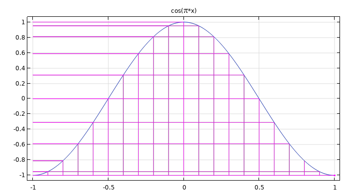A graph that contains a blue line with a parabola-like shape that opens downwards and also includes a series of purple horizontal and vertical lines that display a cross-hatching appearance. Illustration of how points on the x-axis are mapped to the y-axis via the function .

For uniformly sampled points, values close to and  are more likely due to the fact that is almost flat near the points and , which both map to , as well as near the point , which maps to . We thus expect a higher probability density near and , which is reflected in the computed probability function estimates (KDE plots) below.

The polynomials that are orthogonal with respect to a uniform probability distribution on are the Legendre polynomials, denoted .

The first few unnormalized and normalized Legendre polynomials on are listed in the following table:

n
0
1
2
3
4

The normalized Legendre polynomials fulfill the following condition:

Relative to the notation used earlier, we have:

and

Let's compute the expansion up to degree 4

where

We have, for the zeroth-degree coefficient:

where

since we are integrating over a whole period. This is also the mean value of the random function .

In general, for a polynomial chaos expansion with lowest order polynomial equal to , the coefficient is the mean value of the function . In this case:

For the first-degree coefficient:

where

since this is proportional to the average value over a whole period. We can also see that this integral equals zero by noting that we have an even function multiplied with an odd function. The product is an odd function that we then integrate over an interval symmetric around zero, which evaluates to zero.

For the second-degree coefficient:

For the third-degree coefficient we again get zero due to the fact that we are integrating an odd function:

Finally, for the fourth-degree coefficient:

Putting it all together we get:

The figure below shows a comparison between the PCE approximation and the exact function.

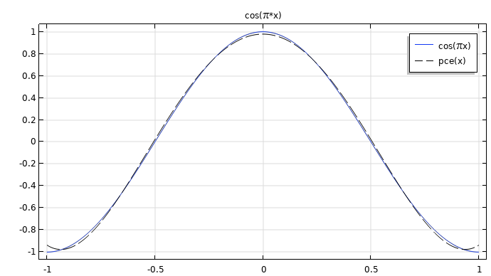
A comparison between the PCE approximation and the original function.

Mean and Variance Calculation

We can use the expansion to compute the variance of .

Recall the definition of variance:

Since earlier, we have that:

and thus:

since the polynomials are orthonormal.

For the expectation value of a random function , we have:

where is the probability density function for . In this case we have:

so that:

For the expectation integrals of the normalized Legendre polynomials, we get:

since they by definition are normalized with respect to the probability density function:

In total, we get for the variance:

The standard deviation is:

For a general polynomial chaos expansion in normalized polynomials, the following relationships hold:

Uncertainty Quantification Module Calculations

For comparison, we can perform an uncertainty propagation analysis for the function . The resulting QoI Confidence Interval table below shows a mean value near zero and a standard deviation of about 0.707, which is consistent with the analytical calculations.

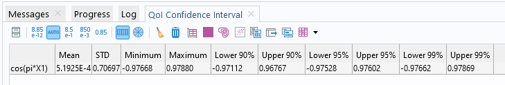
The QoI Confidence Interval table results.

In addition, we can perform direct Monte Carlo simulations using the same technique as covered in the tutorial model based on the Ishigami function.

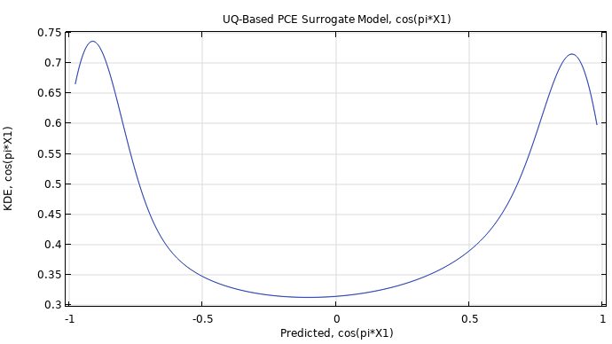
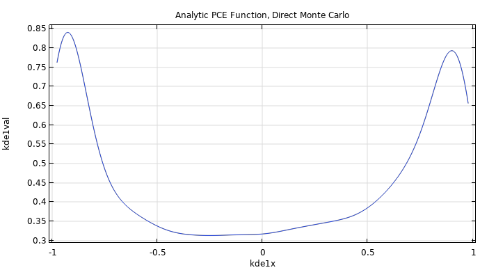
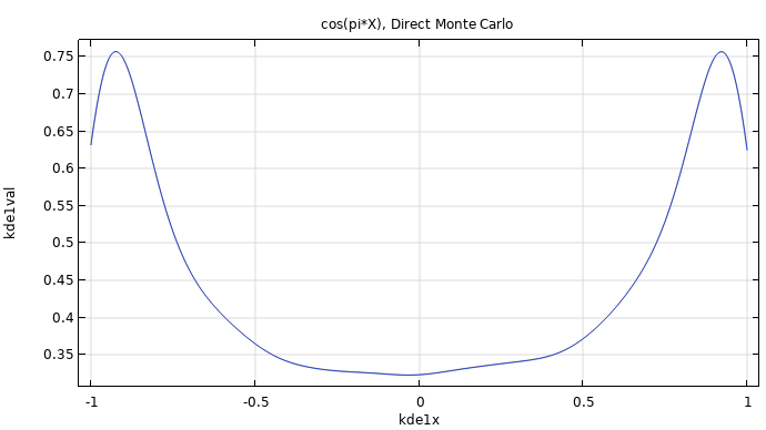
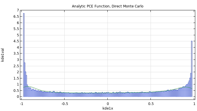
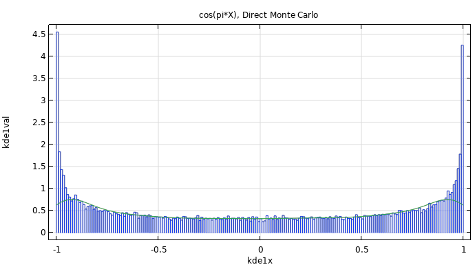
The table below compares the estimated probability distributions (KDE plots) of from two direct Monte Carlo simulations and a UQ-based PCE surrogate model with an uncertainty propagation analysis. For values close to the end points of the interval , the probability distribution shows rapid variations, corresponding to higher frequency content in the probability distribution. These rapid variations are not fully represented by the polynomial expansion. However, the lower frequency content of the distribution is well-represented by the expansion with reasonably accurate values for quantities such as the mean and variance. The built-in automatic PCE regression method can find a good fit using only 200 sample points, whereas the Monte Carlo simulations here use 30,000 sample points. The fact that the built-in PCE surrogate models can be created using orders of magnitude fewer sample points is the main motivating factor for using it instead of direct Monte Carlo simulations. In a case where the model evaluations are not an analytical function, such as , but instead a full-fledged finite element model, it is important to keep the number of model evaluations to a minimum. The default settings for the PCE surrogate model minimize the number of model evaluations.

Plot	Comments
	The figure shows a KDE plot of a PCE surrogate model computed using the Sparse Polynomial Chaos Expansion (SPCE) method in the Uncertainty Quantification Module. This PCE includes higher-degree terms compared to the analytically derived PCE surrogate model, which only includes terms up to degree 4. The PCE fit is based on 200 input points. The corresponding model file is available here.
	The figure shows a KDE plot of a Monte Carlo simulation of the analytically derived PCE, , including terms up to degree 4. The plot is based on 30,000 sample points for , uniformly distributed in . The corresponding model file is available here.
	The figure shows a KDE plot of a Monte Carlo simulation of the function , without approximation. The plot is based on 30,000 sample points for , uniformly distributed in . The corresponding model file is available here.
	The figure shows a histogram plot of a Monte Carlo simulation of the analytically derived PCE, , including terms up to degree 4. The plot is based on 30,000 sample points for , uniformly distributed in . The corresponding model file is available here.
	The figure shows a histogram plot of a Monte Carlo simulation of the function , without approximation. The plot is based on 30,000 sample points for , uniformly distributed in . The corresponding file is available here.