Analyze Thin Structures Using Up and Down Operators

Modeling complex geometries with thin structures can be very costly in terms of computational effort, particularly as such structures require quite a lot of mesh elements in order to resolve them. COMSOL Multiphysics provides dedicated features for modeling thin structures so that such models can be solved efficiently while maintaining accuracy. To set up and postprocess thin structures, COMSOL Multiphysics also provides specialized operators to help you consider all the relevant parameters required for accurate results.

What to Consider When Modeling Thin Structures

COMSOL Multiphysics offers dedicated interfaces and boundary conditions to model thin structures efficiently for a large variety of application areas, including:

• The Thin Layer boundary condition or Heat Transfer in Thin Shells interface for modeling highly conductive or resistive thin layers, like PCB tracks or air gaps.
• The Interior Wall boundary condition in the fluid flow interfaces to model, for example, baffles in a heat exchanger, or the Thin Film Flow interface to model lubrication.
• The Thin Elastic Layer boundary condition or the Shell interface for structural mechanics problems.
• The Electric Currents, Shell interface to model thin conductive layers where inductive effects are negligible.

These features can save a lot of computational effort because they are defined in 2D and are therefore not resolved as 3D objects, which would require a fine mesh resolution. Yet, when you use this type of simplification, you still want to be able to evaluate all of the effects you would consider if you had modeled it in 3D. Let’s have a look at the following example.

Consider a channel with a wire gauze inside it. To model this, you can use the Screen boundary condition for interior boundaries within the CFD Module, which uses correlation functions for the screen resistance and refraction. The underlying equations describe the influence of the screen on the flow field, like the loss in momentum. The picture below represents the flow properties for a pipe with a wire gauze inside.

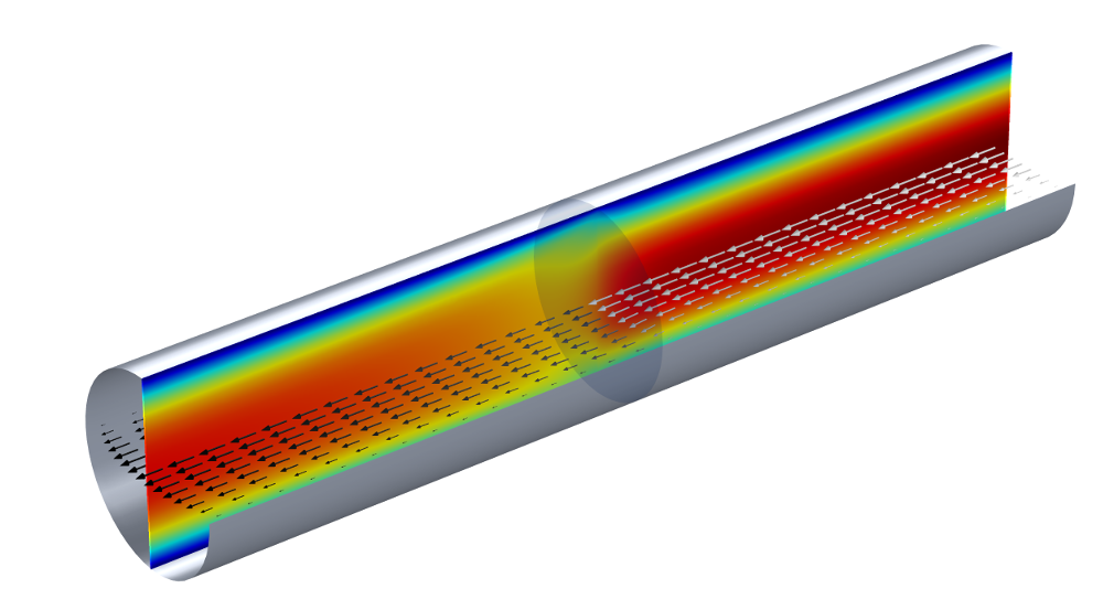
A flow channel with a wire gauze. The color of the slice plot indicates the velocity magnitude. The arrows show the flow direction and their color (grayscale) indicates the pressure. The sharp pressure change at the wire gauze boundary is represented by the arrow color changing from light to dark gray.

A question that arises is: What is the pressure drop across the wire gauze, particularly as we have modeled the gauze as a 2D object?

How to Calculate a Variable Change Across Two Sides of a Boundary

The Screen boundary condition from our example calculates the pressure drop and velocity change. If we take a look at the underlying equation, we can see that the notation uses \mathbf{u}_+ and \mathbf{u}_- to specify the velocity at either side of the gauze. If we also look at the variable for the pressure in the Equation View for the Screen boundary condition, we can see that the expression used to calculate it uses up(p) and down(p), which are the pressure values on each side of the boundary. The up and down operators of the other variables, such as the velocity or density, can also be used to evaluate their values at either side of the internal boundaries.

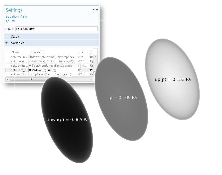
The equation view for the Screen boundary condition and plots for the different pressure variables, using the same gray color scale and with the simulation results for the average pressure.

Let’s have a look at another example: The Shell and Tube Heat Exchanger from the Heat Transfer Application Library. In this case, the Thin Layer boundary condition is used to separate the water flow domain (Domain 1) from the air flow domain (Domain 2). Here, the temperature on the side adjacent to both the water and air domains is of interest in order to calculate the temperature difference over the tubes. COMSOL Multiphysics offers another useful operator for this case — the side operator with the syntax side(entity,expr). So, if we want to evaluate the temperature on the side that is adjacent to the water flow domain, the expression is side(1,T) and analogously, side(2,T) for the air domain.

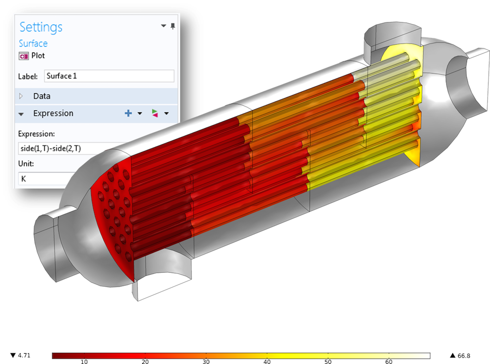
The surface plot showing the temperature difference between the air flow and water flow domains, evaluated with the help of the side operator.

When to Consider Different Directions for the Model Setup

So far, we have seen the use of operators for postprocessing, but how do these operators relate to setting up models? In the following heat transfer example, two domains with low thermal resistance are separated by two highly resistive, but thin, domains (see the figure below). One of these domains also acts as a heat source. The Thin Layer boundary condition with the General formulation can be used for this case. (The General formulation uses an extra dimension, which enables us to apply a heat source on only one side of the internal boundary. Read more about extra dimensions in a previous blog post about multiscale reactors.)

To properly set up the Thin Boundary Layer feature and its Layer Heat Source subfeature, you need to know which side is the downside and which is the upside. In the figure below, three possible setups and their results are compared.

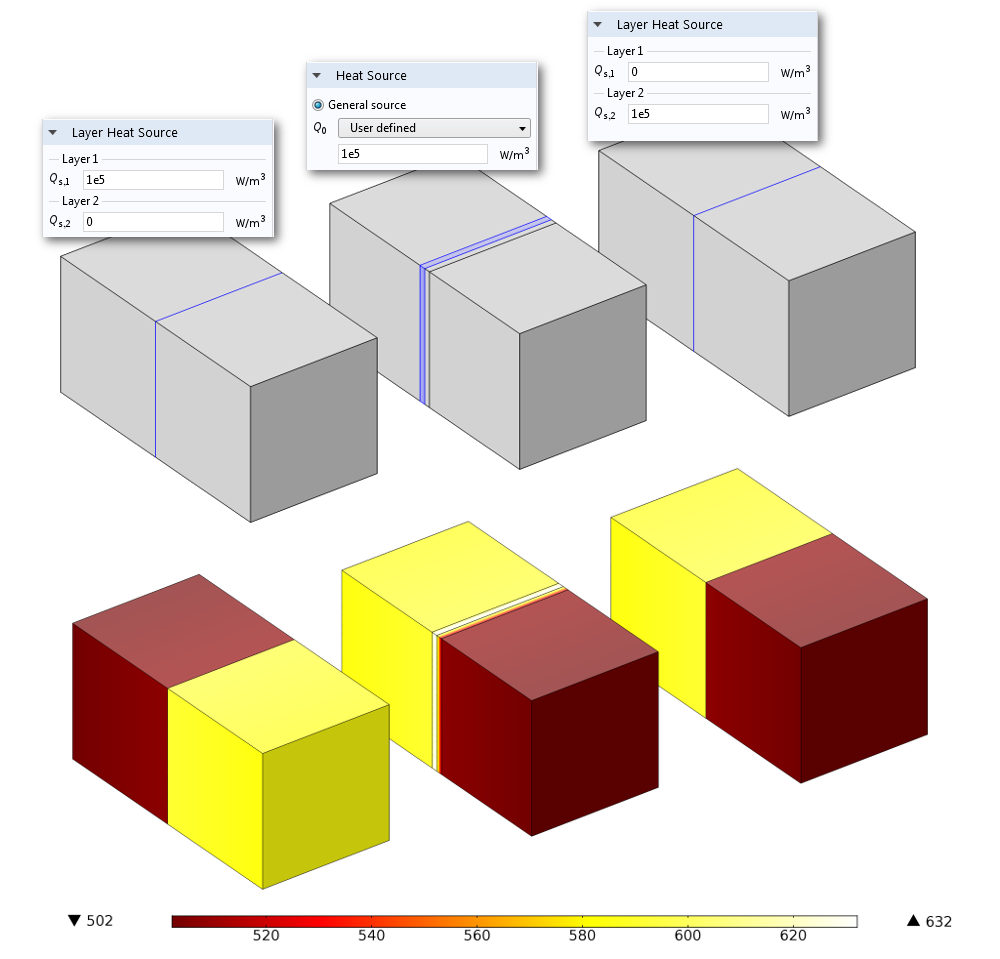
Left: A model using the Thin Layer boundary condition, where a Layer Heat Source subfeature is applied to Layer 1. Middle: A model resolving the two adjacent thin layers as 3D domains, where a Heat Source domain condition has been applied to one of the domains. Right: A model using the Thin Layer boundary condition, where a Layer Heat Source subfeature is applied to Layer 2. The resulting temperature distribution shows that the setup of the Thin Layer boundary condition on the right side, where the Layer Heat Source subfeature is applied to Layer 2, corresponds to the model with the resolved layers in 3D, shown in the middle.

As shown, you can apply a heat source to one side of the internal boundary to simulate heat emanating from a thin layer, but you have to make sure that you apply it to the correct side. The same holds for the definition of the layer thickness and material properties, particularly if the two differ for these properties. Trial and error is an option for defining these scenarios, but with more complex geometries, it takes much longer to solve the model, and if there are numerous thin layers with different properties and heat sources, this is not really a good option. What you need to do is initialize a solution.

I recommend the following procedure:

• Right-click on the Study node and choose Get Initial Value (because you can check if the initial setup is correct at the same time).
• Duplicate the Data Set and add a selection with the Thin Layer boundary condition.
• Create a new 3D Plot group and select the Arrow Surface plot.
• In the expression field, enter the expression for the up (down) components, which is unx,uny,unz (dnx,dny,dnz). Or, with the Thin Layer boundary condition from the Heat Transfer Module, you can choose the corresponding components from the predefined expressions: ht.unx, ht.uny, ht.unz ( ht.dnx, ht.dny, ht.dnz).

With our example, the resulting plot (viewed in the xy-plane) looks like the figure below.

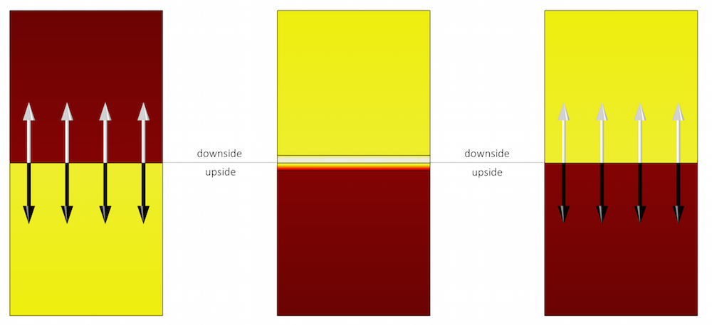
White arrows (unx,uny,unz) point from the upside to the downside, and black arrows (dnx,dny,dnz) point from the downside to the upside. The model that considers the thin layers in 3D has applied the heat source to the downside. For the 2D model, the heat source applied in the Layer Heat Source subfeature must be applied on the downside of the thin layer, which corresponds to Layer 2, since the order of layers is from the upside to the downside.

Concluding Thoughts on Using Up and Down Operators

The different features within the physics interfaces for thin structures enable you to model such structures efficiently. These features use built-in operators to describe physical effects on both sides of the thin layers. You can use these operators to analyze your model and set up the Thin Layer boundary condition in the general form.

If you have questions about using these operators in your simulation, please contact us.