Tsunamis: They’re destructive and fast moving — some traveling as fast as 800 km/h (500 mph)! This natural disaster occurs when a displacement of a mass of water in a body of water, such as an ocean or lake, induces a series of waves. In today’s blog post, we discuss an established benchmark model of a tsunami-inspired experiment that uses the Shallow Water Equations, Time Explicit interface, available with the COMSOL Multiphysics® software as of version 5.6.
1993 Hokkaidō Earthquake
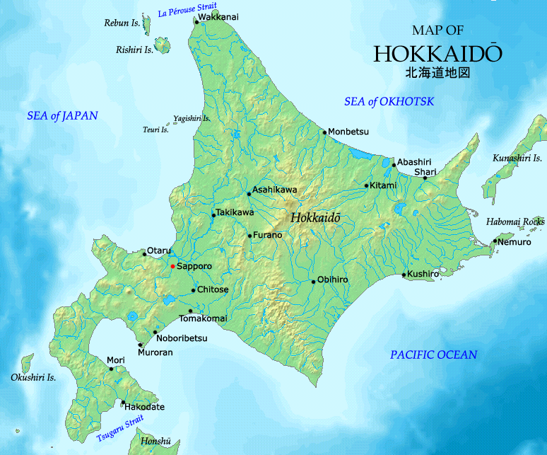
In July 1993, an earthquake with a magnitude of 7.8 on the Richter scale occurred in the Sea of Japan. (For reference, earthquakes with a magnitude of 7.0 to 7.9 happen 10 to 20 times per year and are known to cause severe damage to poorly designed and well-designed structures alike). The quake, often referred to as the 1993 Hokkaidō earthquake, took place 55 km southwest of the island of Hokkaidō, the second largest and northernmost of the main islands of Japan, and 75 km north of the small island of Okushiri.
Note: Since 1900, Japan has experienced 100 earthquakes with a magnitude of 7.0 and above. The largest earthquake recorded in Japan occurred in 2011. The quake, often referred to as the 2011 Tōhoku earthquake, had a magnitude of 9.0 and its effects were felt worldwide.

Map of Hokkaidō. Image licensed under GNU Free Documentation License via Wikimedia Commons.
The earthquake of 1993 triggered several tsunami waves, resulting in extensive damage to both Hokkaidō and Okushiri, especially the latter. In addition, both the southeastern coast of Russia and the eastern coast of South Korea faced the wrath of the tsunami.
Ultimately, this natural disaster resulted in the death of hundreds of people, the destruction of hundreds of homes, and about $600 million in property losses, with a majority of this devastation caused by the tsunami waves.
What made the tsunami so destructive? While in motion, its waves reached massive runup heights, one of which was recorded to be 32 m (~104 ft) high — about 3 times as tall as a telephone pole! The extreme tsunami runup mark was discovered in Monai Valley, a small gulley near the village of Monai on the west coast of Okushiri.
Here, we discuss an established benchmark model for analyzing tsunami runup on an experimental scale…
Analyzing Tsunami Waves and Runup with Simulation
Using numerical simulation and physical experiments, researchers at the Central Research Institute for Electric Power Industry (CREIPI) in Abiko, Japan, were able to recreate a scaled version of the extreme tsunami runup heights generated during the 1993 Hokkaidō earthquake in a large experimental tank (205 m long, 6 m deep, and 3.4 m wide). The bathymetry (depth measurement for oceans, seas, and lakes) of the laboratory model is 1/400 the size of the actual bathymetry of Monai Valley.

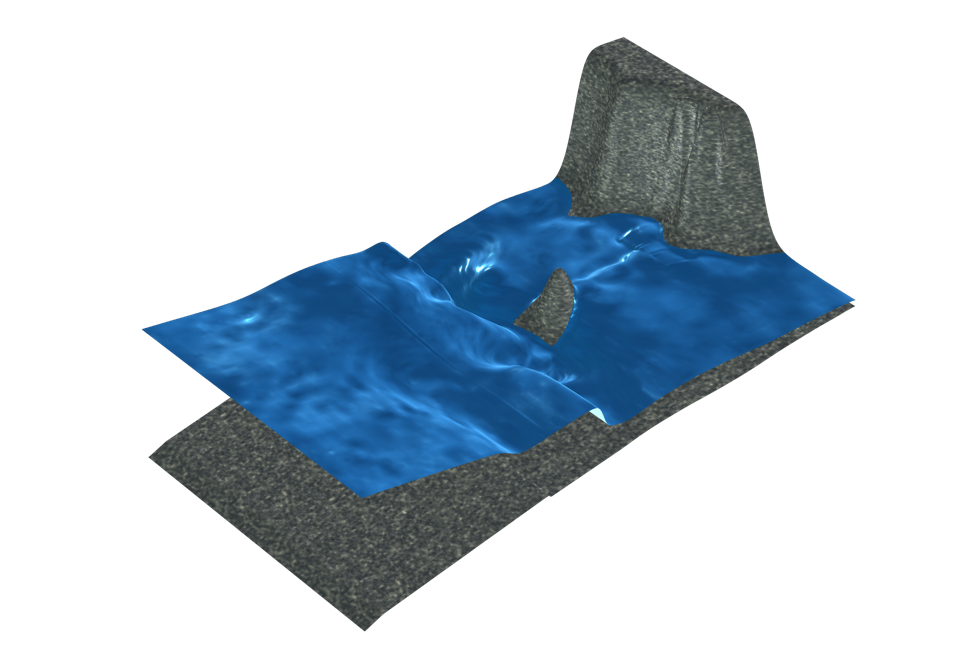
Tsunami Runup onto a Complex 3D Beach, Monai Valley benchmark model.
The Tsunami Runup onto a Complex 3D Beach, Monai Valley benchmark model, shown above, is based on the laboratory work conducted at CREIPI. It simulates a small rectangular region of the CREIPI experimental tank that is 5.445 m long and 3.402 m wide. Like the CREIPI tank, the tank modeled here is filled with still water, and a known incident wave is imposed at one of its boundaries.
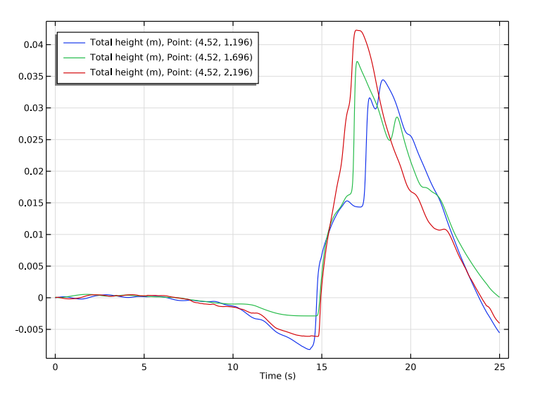
Three Domain Point Probes are included in the model to track the evolution of the water level at three points:
- x = 4.52 m, y = 1.196 m
- x = 4.52 m, y = 1.696 m
- x = 4.52 m, y = 2.196 m
Note: The Shallow Water Equations, Time Explicit interface is used extensively in this work. With this feature, you can use a depth-averaged formulation to solve free-surface flows in 1D and 2D domains and easily define the bottom topography in a model from a digital elevation model.
Next, we’ll go over some of the interesting results from the benchmark model. Feel free to jump ahead to the step-by-step instructions for building this model by downloading it here: “Tsunami Runup onto a Complex 3D Beach, Monai Valley“.
Benchmark Results
Overall, the applied wave makes the shoreline in the model move back and forth, completely covering the small island in the middle of the domain with water in the process.
An animation of the tsunami runup during the simulated experiment.
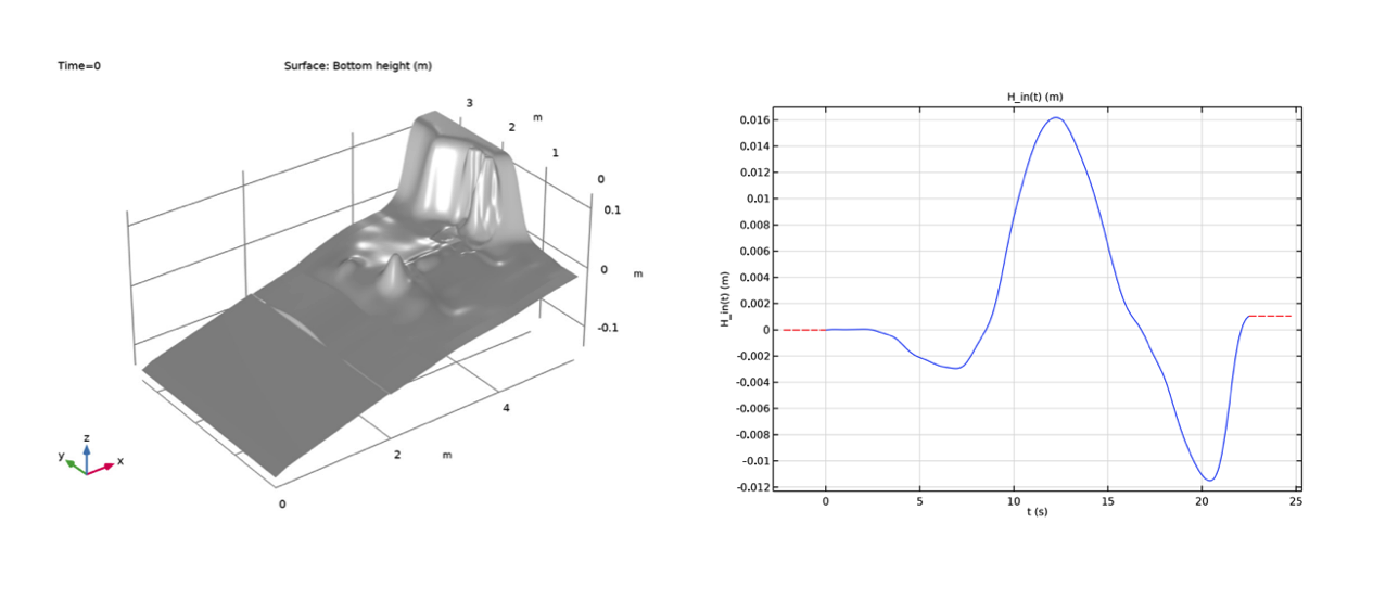
In the images below, you can view the bottom height and profile of the incoming wave.

The bottom topography (left) and profile (right) of the incoming wave.
In the graph below, you can view the calculated water levels at the three domain points. The points see the waves at different times due to the irregularities of the bottom topography. These results agree well with the existing experimental and simulation results in literature (see Reference 3 in the tutorial model documentation).

The National Oceanic and Atmospheric Administration (NOAA) recommends using this type of benchmark model when studying tsunami waves.
Try It Yourself
We jumped right to the results here, but you can learn how to build the Tsunami Runup onto a Complex 3D Beach, Monai Valley model by clicking the button below:
Further Reading
Want to see benchmark models in other fields of study? Check out these blog posts:


Comments (0)