How to Compute Distances Between Objects in COMSOL Multiphysics®

Have you ever modeled deforming objects in the COMSOL Multiphysics® software and wanted to know the distance between them? In today’s blog post, we will look at how to compute distances between objects using methods for determining the closest distance field. We’ll also find out how to use the distance field as a part of a multiphysics model.

Computing Distances with the General Extrusion Component Coupling

Let’s consider two objects labeled A and B, shown below. The three distances that we want to compute are:

1. Distance to object A as a distance field. In this case, we calculate the distance and direction from all of the points surrounding and inside object A to the closest point on its boundary (d_A).
2. Distance from every point on the boundary of object B to the closest point on object A (d_AB).
3. Endpoints of the line that is the shortest distance between objects A and B (d_AB,min).

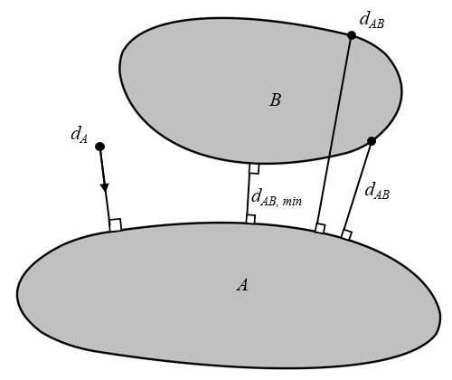
Two objects, A and B, and the distances that we want to compute.

We can compute all of these various distances using a combination of the General Extrusion and Minimum component couplings in COMSOL Multiphysics. Let’s first look at how to use the General Extrusion component coupling. We name the operator A_b and define its Source Selection to be the boundaries of object A. Within the Advanced section, we use the Mesh search method of Closest point. These settings are shown below. All other settings for this operator can be left at their defaults.

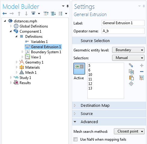
The settings for the General Extrusion component coupling used to compute the closest point distance. Note that the Mesh search method is set to Closest point.

We use this operator within the definition of a variable called d_A, defined as:

sqrt((x-A_b(x))^2+(y-A_b(y))^2)

This variable is defined over the domains where we want to compute the distance field; in this case, just the surrounding domain. We can also compute the negative of the gradient of this distance field, -\nabla d_A(\mathbf{x}). This gives us the components of a vector field that points toward the closest point on the boundary of A. We can use the Differentiation operator d(d_A,x) and d(d_A,y) to take the spatial derivatives, as shown in the screenshot below.

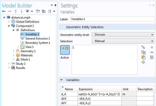
The variable definitions.

We can use these variables anywhere that we want. For example, we can plot the distance field or make material properties dependent upon distance. The image below plots the contours of the distance and the direction vectors. Note that the distance is computed even in the region behind object B. We clearly get quite a bit of information here, but there is a substantial computational cost, since the shortest distance is computed at every point in the surrounding domain. There are also times when we don’t need all of this information and just want the distances between objects.

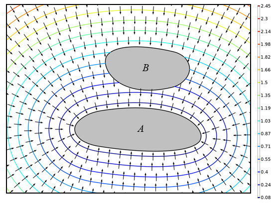
The distance field (contour lines) and shortest direction to the boundary of object A (arrows) in the domain surrounding the two objects.

Calculating Clearances Between Objects

Let’s make things a bit easier and only concern ourselves with the distance between two objects and not the direction. We use the same General Extrusion component coupling, but only need to define a variable on the boundary of object B to compute the distance.

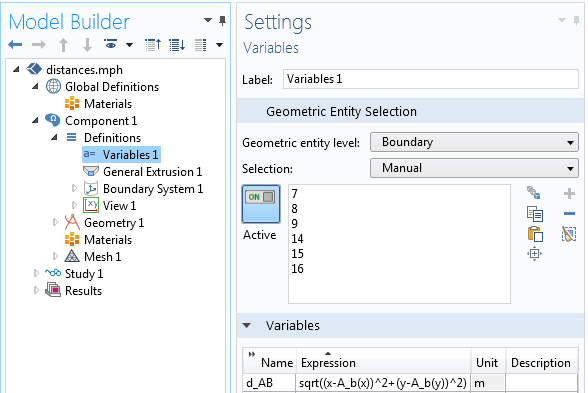
The variable defining the distance between the objects.

While this is the same distance function we used before, we don’t need a mesh in the intermediate space. We don’t even need a mesh over domains A and B; there just needs to be a mesh on the boundaries of the objects. This approach takes much less time, but it gives us only the shortest distance from object A to every point on the boundary of object B. We cannot recover the direction vector. We can also flip all of these definitions around and compute the shortest distance from object B to every point on the boundary of object A. These distances, shown in the plot below, are available along the boundaries of the objects.

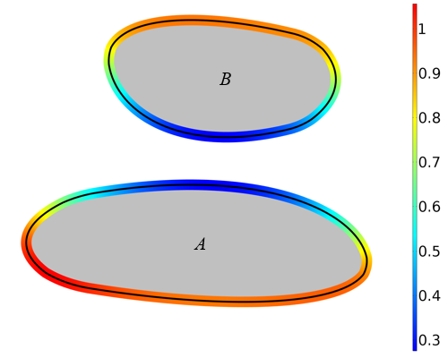
The distance from every point on the boundary of object B to the closest point on object A and vice versa.

Computing the Shortest Line Between Objects Using the Minimum Component Coupling

Now, let’s find the line that describes the shortest distance between the two objects. In the previous section, we saw that we can compute two variables, d_AB and d_BA, which describe the shortest distances between A and B and vice versa. We now want to find the minimum distance between the boundaries of these domains. Thus, we set up two different Minimum component couplings: one for the boundary of object A and another for object B. We call these operators minA and minB, as shown in the screenshot below.

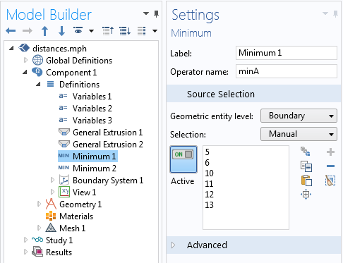
The definition of the Minimum component coupling over the boundary of object A.

We then call these Minimum component couplings to extract the minimum distance. We can also provide a second argument to the Minimum component coupling to find the coordinates at which the distance is at a minimum. For example, by defining the variable A_x as the expression minA(d_BA,x), it takes on the value of the x-coordinate at which d_BA is at a minimum over the boundary of A.

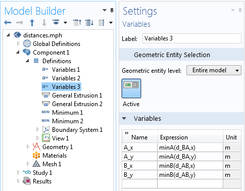
The definitions for the coordinates of the shortest line segment between two domains.

We can call the variables defining these coordinates anywhere we want. For example, we can use the Cut Line feature to show the shortest line segment connecting the two objects, as seen in the following image. If we have a meshed domain and a solution between the two objects, then we can plot the fields just along the shortest line between the two.

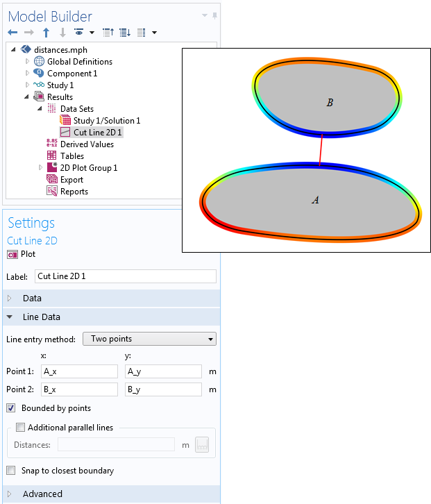
The Cut Line feature, used to determine the shortest line between objects.

Limitations and Uses of Calculating Distances in COMSOL Multiphysics®

These techniques for determining distances can be used in any model. Although the examples presented here are in 2D, they can all be generalized to 3D as well. However, computing the 3D distance field does take a relatively long time, whereas calculating distances between boundaries and clearances is less intensive.

Computing the distance field around nonsmooth shapes also requires a bit more care. As shown in the figure below, the distance field around reentrant corners are nonsmooth, hence the direction vector will be undefined along those lines that are equidistant from two different parts of the boundary. Resolving this nonsmoothness of the distance field requires a finer mesh.

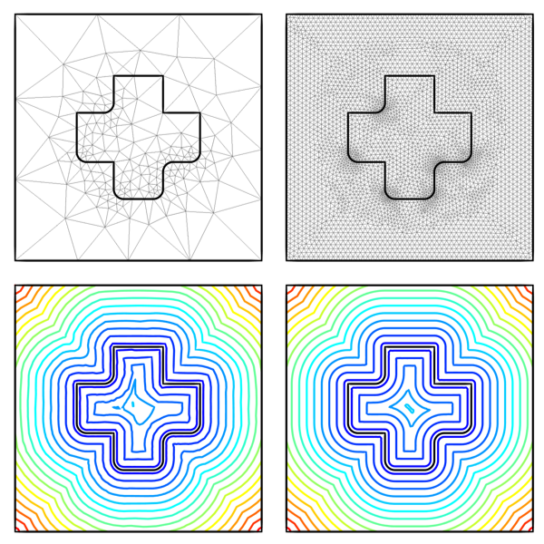
The distance field around and inside an object with reentrant corners on a coarse mesh (left) and a more refined mesh (right). The smoothness of the distance field is mesh dependent in such cases.

Once we have computed this distance field on an appropriately fine mesh, we treat it like any other variable in our model. For example, we can make material properties a function of distance from a surface. The image below shows such a representative material distribution.

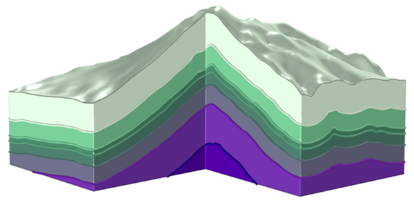
A representative material distribution that is a function of distance to the surface.

It is also possible to use the distance function to help visualize our results. Suppose we are only interested in the part of the solution that is within a specific distance of the surface. In this case, we can use the Filter subfeature when making a volume plot. We then enter a logical expression to only display the results that are within a certain distance of the object’s surface, an example of which is shown below.

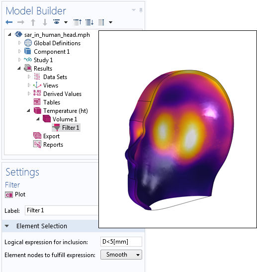
Using the distance function to plot only the solution within 5 mm of the surface.

Concluding Thoughts on Computing Distances Between Objects in COMSOL Multiphysics®

We have demonstrated how to compute a distance field to a boundary within a model, the distances between boundaries, and the shortest line segment between two boundaries. This approach also works to calculate distance fields from edges and points in 3D models. The computed distances can be used anywhere within the setup, physics definitions, and results evaluation of a model. We’ve shared a couple of examples here, but now it’s your turn. We would love to hear what you come up with!

Further Resources

• Find a variety of help resources for modeling in COMSOL Multiphysics:
  • Using the Help Tools in COMSOL Multiphysics® for Modeling Guidance
  • Using the COMSOL Website Resources for Modeling and Software Help