How to Generate Random Surfaces in COMSOL Multiphysics®

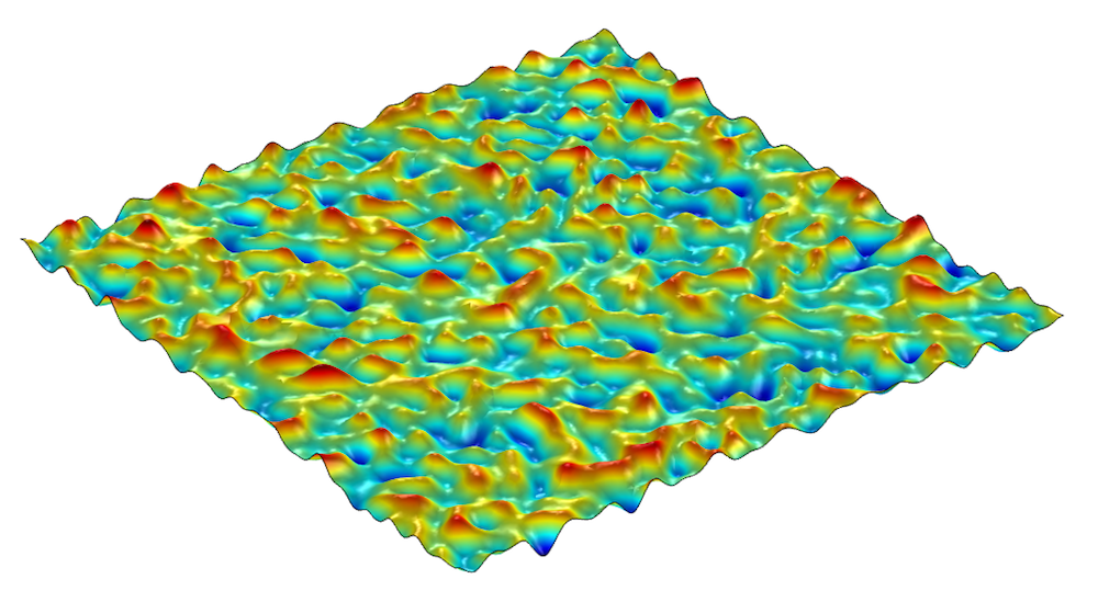
To easily generate random-looking geometric surfaces, the COMSOL Multiphysics® software provides a powerful set of built-in functions and operators, such as functions for uniform and Gaussian random distributions and a very useful sum operator. In this blog post, we show you how to generate a randomized surface with what amounts to a “one liner” expression with detailed control of the constituent spatial frequency components that determine the nature of the surface’s roughness.

Characterizing Surface Roughness

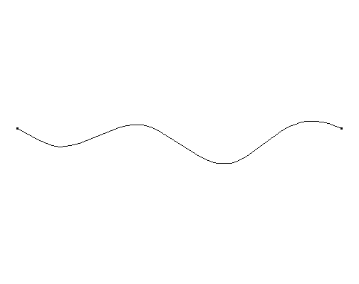
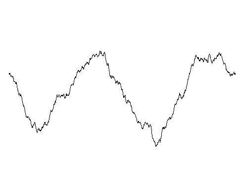
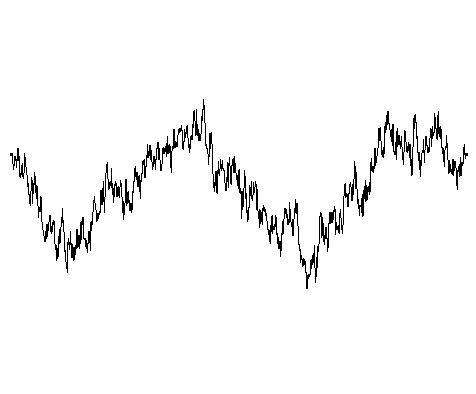
There are many ways to characterize a rough surface. One way is to use its approximate fractal dimension, which is a value between 2 and 3 for a surface. A surface of fractal dimension 2 is an ordinary, almost everywhere smooth surface; the value 2.5 represents a fairly rugged surface; and values close to 3 represent something that is close to “3D space filling”. Correspondingly, a curve of fractal dimension 1 is smooth almost everywhere, the value 1.5 represents a fairly rugged line, and values close to 2 represent something that is close to “2D space filling”.

The range of fractal dimension values for curves going from 1 (left) to about 1.2 (center) and to 1.6 (right).

Using a fractal dimension measure can be a useful approximation, but we need to remember that real surfaces aren’t fractal in nature over more than a few orders of magnitude of scale. Real surfaces have a spatial frequency “cutoff” due to their finite size and due to the fact that when “zooming in”, you will eventually hit some new type of microstructure behavior.

Another way of characterizing surface roughness is with respect to its spatial frequency content. This can be turned into a constructive method of synthesizing surface data by using a sum of trigonometric functions similar to a Fourier series expansion. Each term in such a sum represents a certain frequency of oscillation through space. This is the method that we will use here. Let’s quickly review the concepts of spatial frequencies and elementary wave shapes before moving on to trigonometric series.

Spatial Frequencies

In physics, the frequency of oscillations over time occurs in mathematical expressions like

where the unit of the frequency f is 1/s, also known as hertz or Hz.

Oscillations through space have a corresponding spatial frequency, as in the following expression, where we simply have replaced the time variable t by a spatial variable x and the time frequency f with the spatial frequency v.

where the SI unit of the spatial frequency is 1/m.

Spatial frequencies are commonly represented by a wave number k = 2πv.

A related quantity is the wavelength \lambda=\frac{1}{\nu}, which is related to the frequency and wave number as follows:

There may be more than one dimension of space and, accordingly, there may be multiple spatial frequencies. In 2D, using Cartesian coordinates, we have:

where \bf{k}=(k_x,k_y)=(2\pi \nu_x,2\pi\nu_y) is the wave vector and \bf{x}=(x,y).

The wave vector \bf{k} represents the direction of the wave.

Elementary Waves

A rough surface f(x,y) can be seen as composed of many elementary waves of the form

where φ is a phase angle.

The phase angle also makes it possible to express sine functions due to the relationship sin(\theta)=cos(\pi/2-\theta).

For a completely random surface, it should hold that the phase angle φ can take any value in, say, the interval 0 to π or –π/2 to π/2. When synthesizing elementary waves for a random surface, we can pick φ from a uniform random distribution in such an interval of length π, since we then allow for the expression cos(\phi) to span all possible values between -1 and +1. Note that there may be end-point or wrap-around effects if we choose an interval with a size bigger than π. This is due to the cosine function being its own mirror image in steps of π, according to cos(\pi-\theta)=-cos(\theta).

In order to get an efficient representation that can be used for simulations, we will only allow for a discrete set of spatial frequencies:

ν_x = m, ν_y = n

where m and n are integers.

Let’s consider a surface that is composed of elementary waves of the following form:

By letting m and n take both positive and negative values with equal probabilities, we should be able to get a method of synthesizing a surface with no preferred direction of oscillations.

Note that, in this way, each wave direction is represented twice. For example, the direction (-2,-3) is the same as (2,3); (2,-1) is the same as (-2,1); and so on.

If we allow the spatial frequencies m and n to take values up to maximum integers M and N, respectively, then this corresponds to a high-frequency cutoff at:

Since we also allow for negative values, there are negative cutoffs at:

Having a spatial frequency cutoff at \nu_{xmax}=M in the x direction means that the shortest wavelength we can represent is \lambda_{xmin}=\frac{1}{M}, and similarly for the y direction, \lambda_{ymin}=\frac{1}{N}.

Associated Amplitudes for Elementary Waves

Each elementary wave will have an associated amplitude so that each constituent wave component has the following form:

The final surface will be a sum over such wave components:

The simplest choice of amplitude would be to choose the coefficients A_mn from a uniform or perhaps Gaussian distribution. However, it turns out that this will not generate a particularly natural-looking surface. In nature, different processes, such as wearing and erosion, make it more likely that slow oscillations have a larger amplitude than fast ones. In the discrete case, this corresponds to the amplitudes tapering off according to some distribution:

where the spectral exponent β indicates how quickly higher frequencies are attenuated. Following The Science of Fractal Images (Ref.1), the spectral exponent can be related to the fractal dimension of a surface, but only for an infinite series of waves covering arbitrarily high frequencies and only for certain ranges of the exponent. In practice, the amplitudes a(m,n) of our synthesized surface will be generated using a limited number of frequencies, multiplied with a random function g(m,n) having a Gaussian distribution:

a(m,n) = g(m,n)h(m,n)

A Gaussian, or normal, distribution is chosen to get a smooth but random variation in amplitudes with no limit on the magnitude.

The phase angles φ will be sampled from a function u with a uniform random distribution between –π/2 and π/2:

φ(m,n) = u(m,n)

Summing It Up

To represent our rough surface, we want to use the following double sum:

where x and y are spatial coordinates; m and n are spatial frequencies; a(m,n) are amplitudes; and φ(m,n) are phase angles. This expression is similar to a truncated Fourier series. Although the series is expressed in terms of cosine functions, the phase angles make it so this sum can express a quite general trigonometric series due to the angle sum rule:

Determining Periodicity

Due to its definition, the function f(x,y) will be periodic. In order to get a natural-looking surface, we should “cut out” a suitably small portion by letting x and y vary between some limited values; otherwise, the periodicity of the synthesized data will be apparent. What should these values be?

The overall periodicity will be determined by the slowest oscillations, which correspond to the spatial frequencies m = 1 or n = 1 in the x direction and y direction, respectively. This gives a period length of 1 in each direction.

We could generate the surface over a rectangle [a, a + 1] × [b, b + 1] or smaller in order to “avoid” the periodicity.

Defining Parameters and Random Functions in COMSOL Multiphysics®

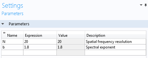
For the COMSOL Multiphysics implementation, start by defining a couple of parameters for the spatial frequency resolution and spectral exponent according to the following figure:

The amplitude generation will require a random function with a Gaussian distribution in two variables. This functionality is available under the Global Definitions node:

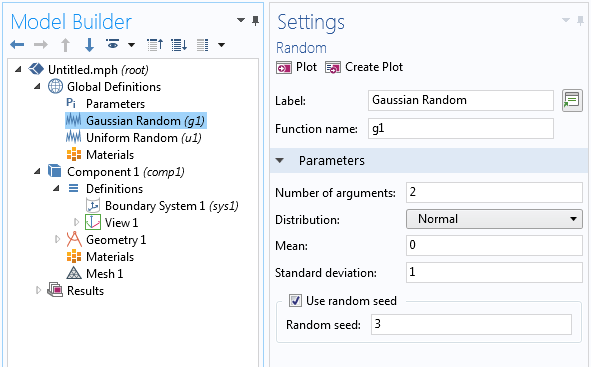
Here, the Label and Function name have been changed to Gaussian Random and g1, respectively. In addition, the Number of arguments is set to 2 instead of the default 1 and the Distribution type is set to Normal, which corresponds to a normal or Gaussian distribution.

In a similar way, for the phase angle, we need a uniform random function in the interval between –π/2 and π/2:

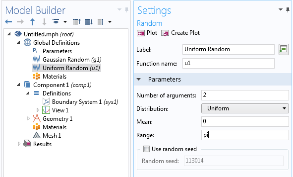
The Label is changed to Uniform Random, the Function name to u1, the Number of arguments to 2, and the Range to pi.

You can optionally use random seeds to get the same surface each time you use the same input parameters.

Defining the Parametric Surface

The next step is to add a Parametric Surface node under Geometry using a fairly lengthy z-coordinate expression, as follows:

0.01*sum(sum(if((m!=0)||(n!=0),((m^2+n^2)^(-b/2))*g1(m,n)*cos(2*pi*(m*s1+n*s2)+u1(m,n)),0),m,-N,N),n,-N,N)

where x = s1 and y = s2 vary between 0 and 1.

The factor 0.01 is used to scale the data in the z direction. Alternatively, this scaling factor can be absorbed into the amplitude coefficients.

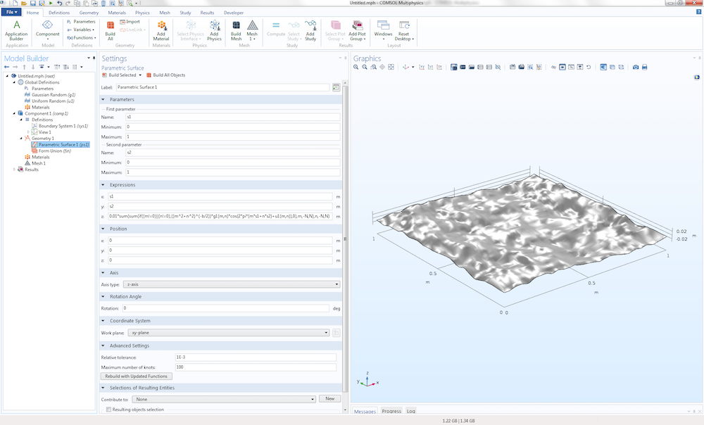
A parametric surface geometry feature is used to generate a synthesized random surface.

Note that whenever you update any of the parameters or expressions for the Parametric Surface, you need to click the Rebuild with Updated Functions button in the Advanced Settings section of the Settings window.

This expression is a double-sum over the integer parameters m and n each running from –N to N. If we compare this to the mathematical discussion earlier, we can see that we have set M = N, resulting in a square surface patch. The term where m and n are simultaneously zero corresponds to an unwanted “DC” term and is eliminated from the sum by the if statement.

The syntax for the sum() operator is as follows:

sum(expr,index,lower,upper)

which evaluates a sum of a general expression expr for all indices index from lower to upper.

The syntax for the if() operator is as follows:

if(cond,expr1,expr2)

for which the conditional expression cond is evaluated to expr1 or expr2 depending on the value of the condition.

In this example, the resolution of the parametric surface has been increased by setting the Maximum number of knots to 100 (the default is 20). In addition, the Relative tolerance is relaxed to 1e-3 (the default is 1e-6). The underlying representation of the parametric surface is based on nonuniform rational B-splines (NURBS). More knots correspond to a finer resolution of the NURBS representation. The tolerance is increased, since we are not overly concerned about the approximation accuracy of the generated surface for this example.

By generating a mesh, we can get a useful visualization of the surface, as seen in the figure below.

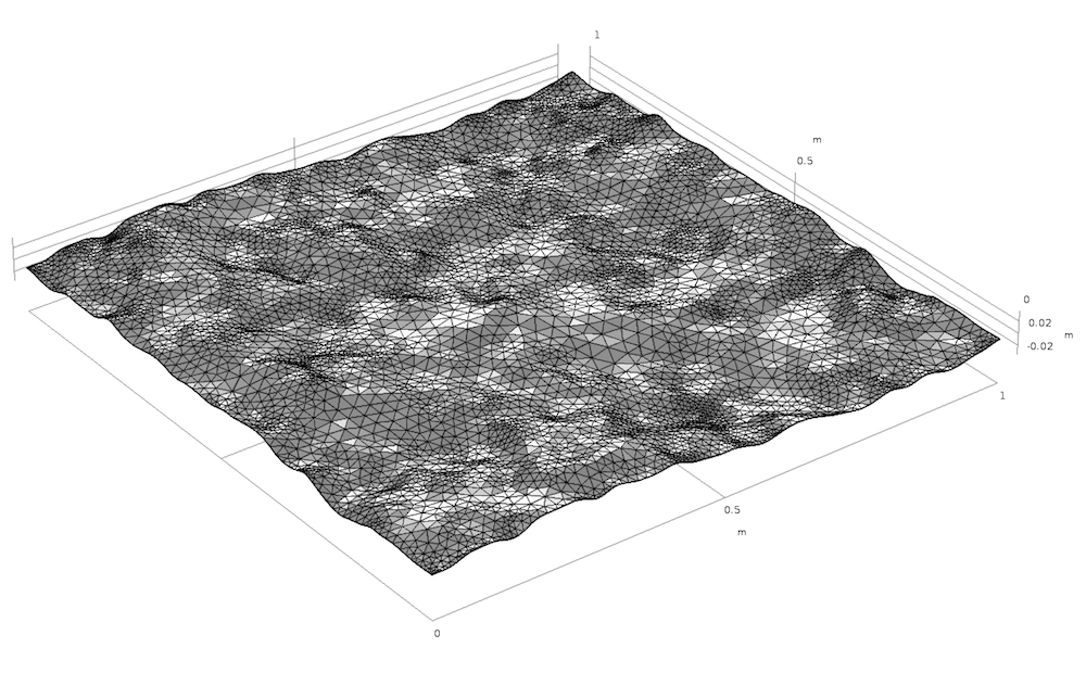
A meshed random surface.

Note that N = 20 means that the fastest oscillations are 1/20 = 0.05 m, assuming SI units. The periodicity in the x and y directions can be seen by following the curves parallel to the y– and x-axes at x = 0, x = 1 and y = 0, y = 1; respectively.

To see the periodicity even more clearly, we can plot the surface on the square [0,2] × [0,2]:

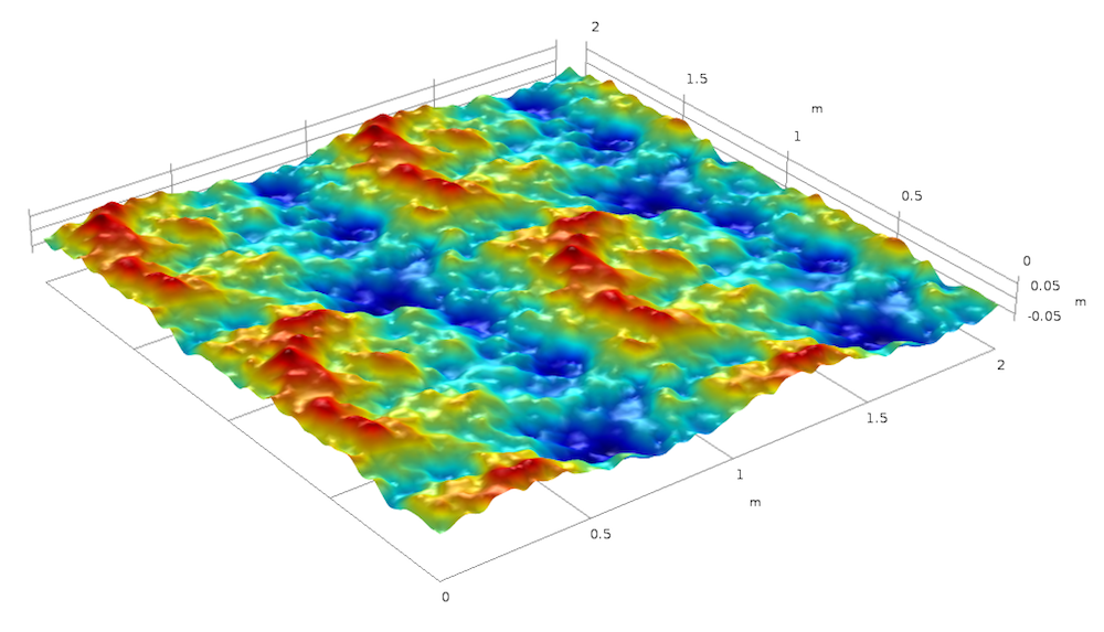
The periodicity of the surface on the square [0,2] × [0,2]. The surface height is represented by color.

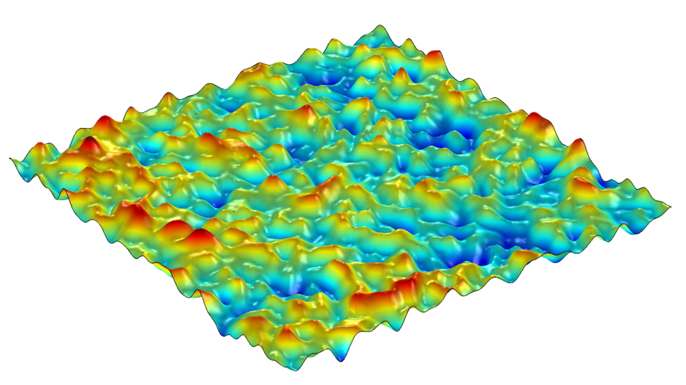
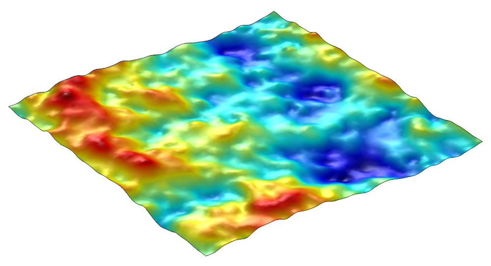
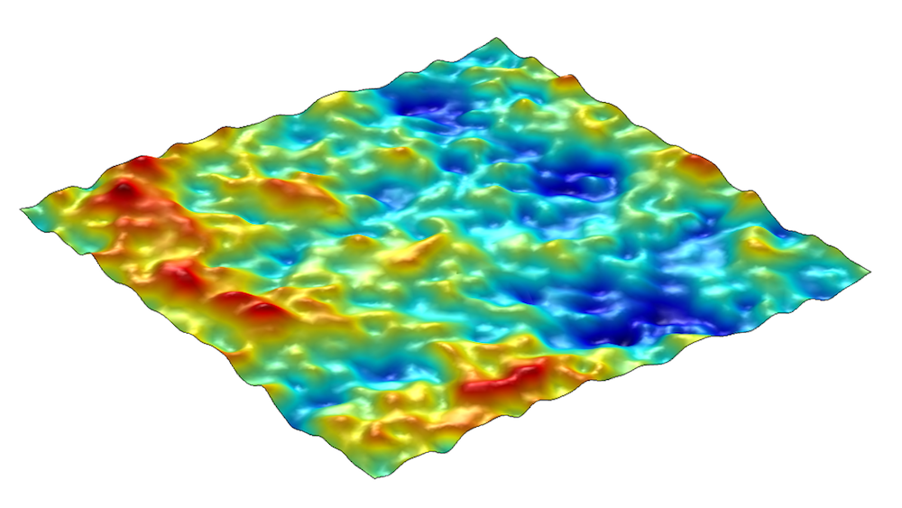
Surfaces generated on the square [0,1] × [0,1] by superimposing 20 frequency components with amplitude spectral exponents β = 0.5, β = 1.0, β = 1.5, and β = 1.8, clockwise from the top-left image. The surface height is represented by color.

Using the Surface Data in Analyses

This type of randomly generated surface can, in COMSOL Multiphysics, be used in any kind of physics simulation context, including for electromagnetics, structural mechanics, acoustics, fluid, heat, or chemical analysis. The expression for the double sum is not limited for use in geometry modeling, but can also be used for material data, equation coefficients, boundary conditions, and more. Using methods, a large number of surface realizations can be used in a loop to gather statistics of the results.

By generalizing the double-sum to a triple-sum, you can synthesize 3D inhomogeneous material data. However, you have to be prepared for long and memory-intensive computations when performing triple-sums for 3D simulations.

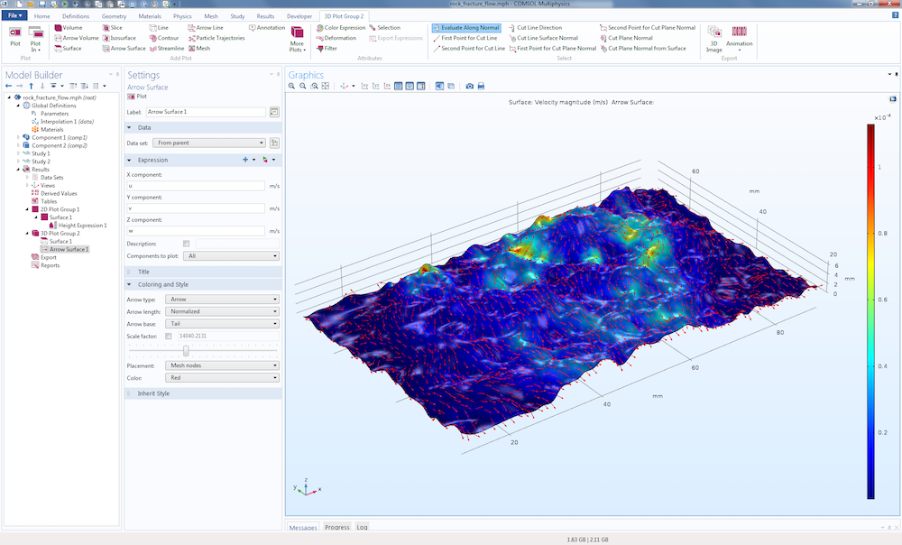
A fracture flow simulation based on synthetically generated fracture aperture data. The Rock Fracture Flow tutorial model is part of the COMSOL Multiphysics Application Library.

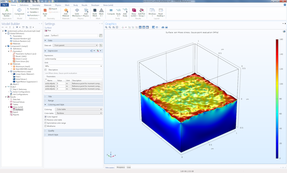
A generic thermal expansion analysis of two 1-centimeter-sized metal blocks with a material interface based on the parametric surface described in this blog post. The bottom material slab is aluminum and the top material slab is steel. The visualization shows the von Mises stress at the material interface and on the surface of the aluminum slab.

Relationship to Discrete Cosine and Fourier Transforms

The sum

is similar to a discrete cosine transform or to the real part of a discrete Fourier transform:

where the subscript c is used to indicate complex quantities and x and y now take discrete values. Here, the phase angle information is encoded in the complex Fourier coefficients.

Due to the definition of the discrete Fourier transform, we are allowed to perform a shift in index in order to generate the following more familiar form:

or by using discrete values:

More commonly, the discrete Fourier transform is indexed like this:

where

Note that in order to generate real-valued data, the Fourier coefficients need to fulfill conjugate symmetry relationships in order to eliminate the imaginary-valued contributions from sine functions. Using a sum of cosine functions (i.e., a cosine transform) avoids this problem.

A fast way of generating a large number of Fourier coefficients is to use a fast cosine transform (FCT) or fast Fourier transform (FFT). This could be done in another program and then imported to the COMSOL Desktop® user interface as an interpolation table. The trigonometric interpolation method described above is slower, but has the advantage that it can be used directly on an unstructured mesh and is automatically refined by simply refining the mesh in the user interface.

For a description of using FFT for synthesizing surfaces, see Ref.1.

1D and Cylindrical Cases

Let’s conclude with a few interesting, special cases of random surface generation in COMSOL Multiphysics, including curves and cylinders.

Random Curve

In a 2D simulation, a random curve can be generated using the following expression:

0.01*sum(if((m!=0),((m^2)^(-b/2))*g1(m)*cos(2*pi*m*s+u1(m)),0),m,-N,N)

where g1 and u1 are 1D random functions.

Note that when generating a curve, the spectral exponent will have a lower value as compared to that of a surface for the “same level of randomness”.

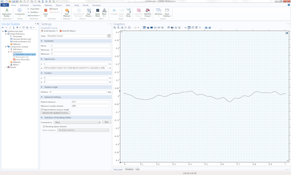
A randomized curve with spectral exponent 0.8.

Random Polar Curve

A randomized curve in polar coordinates representing random deviations from a circle can be generated:

x=cos(2*pi*s)*(1+0.1*sum(if((m!=0),((m^2)^(-b/2))*g1(m)*cos(2*pi*m*s+u1(m)),0),m,-N,N))

y=sin(2*pi*s)*(1+0.1*sum(if((m!=0),((m^2)^(-b/2))*g1(m)*cos(2*pi*m*s+u1(m)),0),m,-N,N))

This corresponds to a parametric curve in 2D polar coordinates:

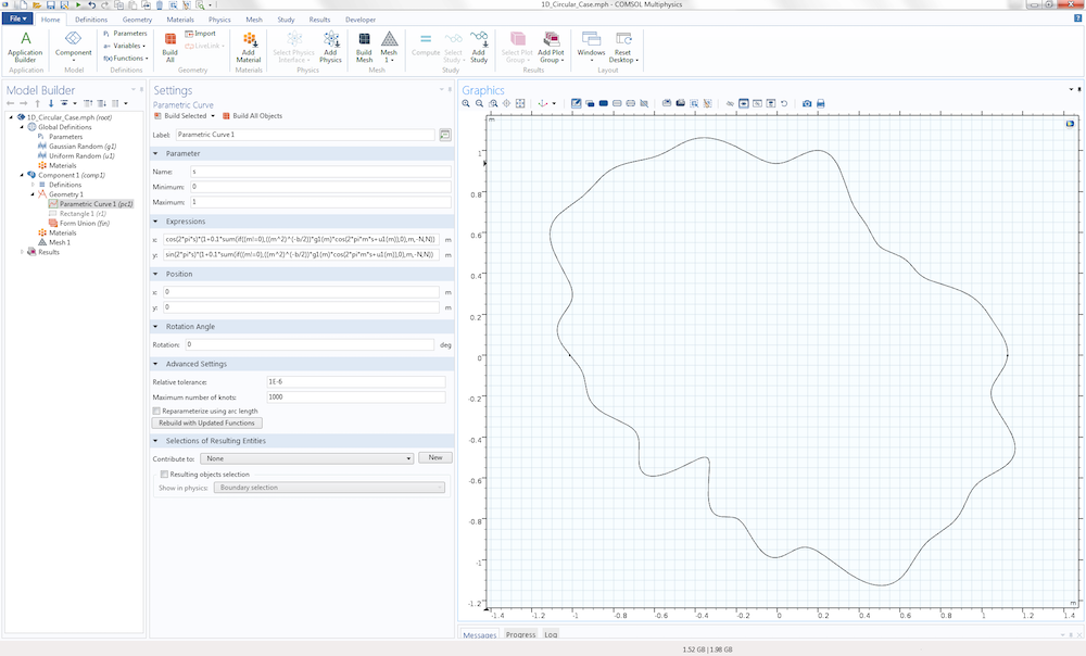
A randomized polar curve with spectral exponent 0.8.

Random Cylinder

A randomized cylinder in 3D can be generated using a parametric surface with parameters as follows:

x=cos(2*pi*s1)*(1+0.1*sum(sum(if((m!=0)||(n!=0),((m^2+n^2)^(-b/2))*g1(m,n)*cos(2*pi*(m*s1+n*s2)+u1(m,n)),0),m,-N,N),n,-N,N))

y=sin(2*pi*s1)*(1+0.1*sum(sum(if((m!=0)||(n!=0),((m^2+n^2)^(-b/2))*g1(m,n)*cos(2*pi*(m*s1+n*s2)+u1(m,n)),0),m,-N,N),n,-N,N))

z=s2*2*pi

where the parameters s1 and s2 vary between 0 and 1.

This corresponds to a parametric surface in cylindrical coordinates:

Such a single-piece random cylinder represents a type of self-intersecting surface that is not allowed in COMSOL Multiphysics. You can easily get around this by, for example, creating four surface patches corresponding to the parameter s1 varying from 0 to 0.25, 0.25 to 0.5, 0.5 to 0.75, and 0.75 to 1.0. One such patch corresponds to a polar angle span of size \frac{\pi}{2}.

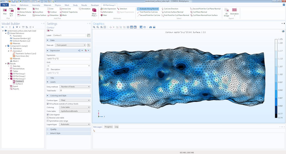
A randomized tubular surface using polar coordinates.

New Part in COMSOL Multiphysics® Version 5.5

As of version 5.5, the Part Library for COMSOL Multiphysics has been extended with several new parts, including a part for creating a random flat surface.

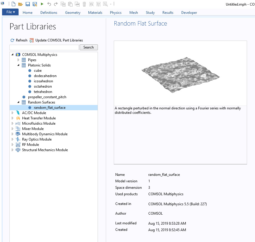
The Random Flat Surface part in the Part Library in COMSOL Multiphysics.

Reference

• The Science of Fractal Images, Editors: Peitgen, Heinz-Otto, Saupe, Dietmar. Eds.