How to Model Conductors in Time-Varying Magnetic Fields

One of the more common uses of the AC/DC Module, an add-on to the COMSOL Multiphysics® software, is for modeling conductors and other lossy materials in time-varying magnetic fields when there are significant induced currents. The appropriate modeling approach depends upon how quickly the magnetic fields vary over time. Here, we review the basics and describe various modeling techniques to use.

Describing the Skin Effect Using the AC/DC Module

Whenever a lossy material, such as a conductor, is exposed to a time-varying electromagnetic field, there will be currents induced in that material. These currents then produce a magnetic field that alters the current distribution within the material, with the net result being that the induced currents will preferentially flow at the surfaces of any lossy material. This is known as the skin effect.

We can model this effect using the AC/DC Module and any of the physics interfaces that solve for the magnetic fields and currents, such as the:

• Magnetic Fields interface
• Magnetic and Electric Fields interface
• Magnetic Field Formulation interface
• Rotating Machinery Magnetic interface

All of these physics interfaces support modeling in the frequency domain under the assumption that the magnetic fields, and all other fields, are varying sinusoidally in time. The Magnetic Fields interface — as well as the Rotating Machinery Magnetic and the Magnetic Field Formulation interfaces — support full time-domain analysis, where the fields can vary nonsinusoidally over time.

Frequency-Domain Simulations for Conductors in Time-Varying Magnetic Fields

To start off, we focus on the frequency domain, a very reasonable thing to do, since most electric devices operate at a known frequency or range of frequencies. Based upon the operating frequency, we can then compute the skin depth, δ, in the material:

where \omega is the operating frequency, \mu_0 is the permeability, \epsilon_0 is the permittivity of free space, \mu_r and \epsilon_r are the relative permeability and permittivity of the material, and \sigma is the material electrical conductivity.

For conductors, this equation can be simplified to:

Strictly speaking, the skin depth is defined in terms of the exponential decrease in the induced currents within a planar, semi-infinite conductor, but it is still a useful measure regardless of the shape of the geometry. First, we always estimate the skin depth of all of the materials in the simulation, since this value governs how we will model them. To understand this key point, let’s look at a simple case of a closed loop of wire (with a wire radius of 1 cm and loop radius of 10 cm) exposed to a uniform background magnetic field at different frequencies, as shown schematically below.

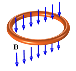
A loop of copper wire exposed to a sinusoidally time-varying magnetic field.

The above illustrated problem can be modeled using a 2D axisymmetric model, as seen below. The infinite element domain is used to truncate the modeling space for the reasons outlined in this previous blog post.

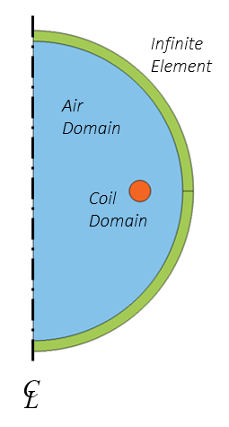
A schematic of the coil model.

Let’s look at the results at several different frequencies. The image below shows the magnitude of the current flow in the coil. At higher frequencies, we can observe how the current primarily flows near the surface of the coil. In fact, at the highest frequency, the current in the center of the coil is, for all practical purposes, zero. That is, the skin effect has shielded the inside of the conductor.

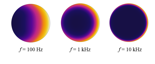
The current flow within the coil cross section at different frequencies.

To appropriately model these various cases, we also need to be aware of the finite element mesh used. At higher frequencies, as the current is being driven closer and closer to the boundaries, we need to have a finer mesh to resolve the spatial variation of the fields. However, the fields are only varying strongly in the direction normal to the boundary and varying quite gradually along the perimeter of the coil.

In these cases, it is appropriate to use the boundary layer meshing functionality, which will insert thin elements normal to the boundary, as shown in the image below. Depending upon how accurately you want to resolve the current distribution in the coil, you can adjust the thickness of the boundary layer elements to be between one half to one skin depth and use as few as two or as many as eight or more boundary layer elements. On the other hand, at frequencies that are low enough, the boundary layer meshing is not needed at all.

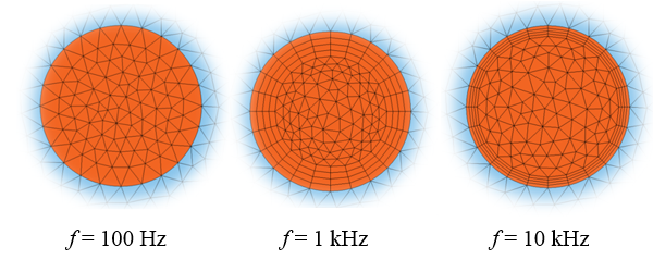
The mesh within the wire at varying frequencies, corresponding to the previous plots of current distribution.

Equivalent Boundary Conditions

Now, we can also see from the image above that at higher frequencies, the current distributions extend very negligibly into the coil interior. Therefore, for all practical purposes, we can say that at frequencies that are high enough, the currents flow on the surface. In these cases, we can use the Impedance boundary condition and not model any of the coil interior at all, as shown in the image below.

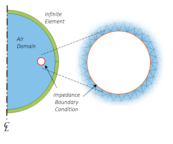
Schematic and mesh of a model using the Impedance boundary condition.

This approach saves us a significant amount of computational effort, since we now only need to mesh the air domain and apply the Impedance boundary condition. Obviously, we do lose some information here: the current distribution within the conductor. But if we do not care about that, then this approach can be a superior alternative to meshing the conductor interior. The first plot below shows the losses in the coil versus frequency, computed via the Impedance boundary condition and via a domain model of the coil with a boundary layer mesh.

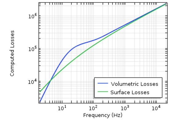
Plot of the computed losses via a domain model and the Impedance boundary condition.

The next figure plots the ratio of the losses computed by using the Impedance boundary condition to the losses computed by explicitly modeling the domains, and this ratio is plotted against the ratio of the wire radius to the skin depth. As the characteristic dimension of the parts (in this case, the radius) approaches ten times the skin depth, the losses computed via these two approaches are similar.

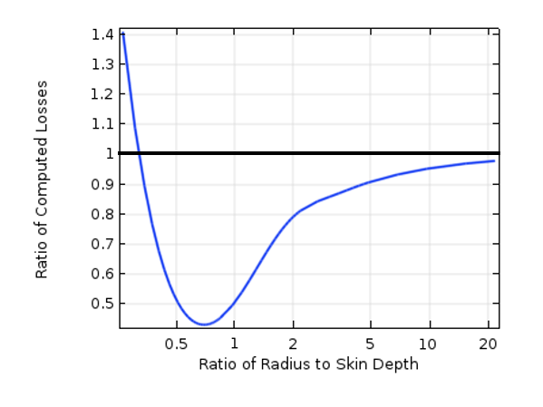
Plot of the ratio of computed losses versus the ratio of object size to skin depth.

We can conclude from the plot above that the Impedance boundary condition gives us an accurate prediction of total losses as long as the skin depth is relatively small compared to the dimensions of the conductors that we want to model. This is an important result, as it can significantly simplify a lot of our frequency-domain modeling within the AC/DC Module.

Time-Domain Simulations for Conductors in Time-Varying Magnetic Fields

Let’s finish up this topic by addressing time-domain simulations. The Impedance boundary condition is not available in this case, since this boundary condition is formulated based upon the frequency-domain form of Maxwell’s equations. For time-domain simulations, we must model and mesh the interior of all conductors. Boundary layer meshing is still appropriate, but you will want to adjust the thicknesses of the elements based on both the average and maximum expected frequency content of your time-domain excitations. This can sometimes lead to a much more computationally expensive model, of course, so try to model in the frequency domain as much as possible.

And what if you have materials that are nonlinear with respect to field strength or materials that you might think you have to model in the time domain? What do you do then? If you’re imagining a ferromagnetic material with a nonlinear magnetic permeability, you can still model the magnetic material in the frequency domain using the effective H-B curve functionality.

Closing Remarks

Having a good understanding of how to model conductive, lossy materials interacting with time-varying magnetic fields is important for effective use of the AC/DC Module. You can either explicitly model the conductive domains or model the conductors via the Impedance boundary condition at higher frequencies. If you do model the domains explicitly, you will need to use a boundary layer mesh to give a good resolution of the currents at higher frequencies, which does increase the computational requirements. If you use the Impedance boundary condition, you introduce an approximation, but you will not need to model the interior of the conductor domains at all, saving you significant computational resources.

Next Steps

To learn more about the specialized features and functionality for electromagnetics modeling available in the AC/DC Module, click the button below.

Additional Resources

To work through a set of supplemental exercises on this topic, see the following tutorials:

• Iron Sphere in a 60 Hz Magnetic Field
• Iron Sphere in a 20 kHz Magnetic Field
• Iron Sphere in a 13.56 MHz Magnetic Field
• Mutual Inductance and Induced Currents Between Single-Turn Coils