How to Model the Compression of a Hyperelastic Foam

To characterize hyperelastic materials, we need experimental data from a variety of tests, including subjection to uniaxial tension and compression, biaxial tension and compression, and torsion. Here, we show how to model the compression of a sphere made of an elastic foam using tension and compression test data obtained via uniaxial and equibiaxial tests. We demonstrate the use of the compressible Storakers hyperelastic material model for computation as well as how force-versus-stretch relationships are calculated for uniaxial and equibiaxial tests.

Using Measured Test Data for Compression Analyses

The figure below shows a schematic view of uniaxial and equibiaxial tension and compression tests. While we don’t discuss the setup required to conduct such tests here, we assume that such experimental data is available.

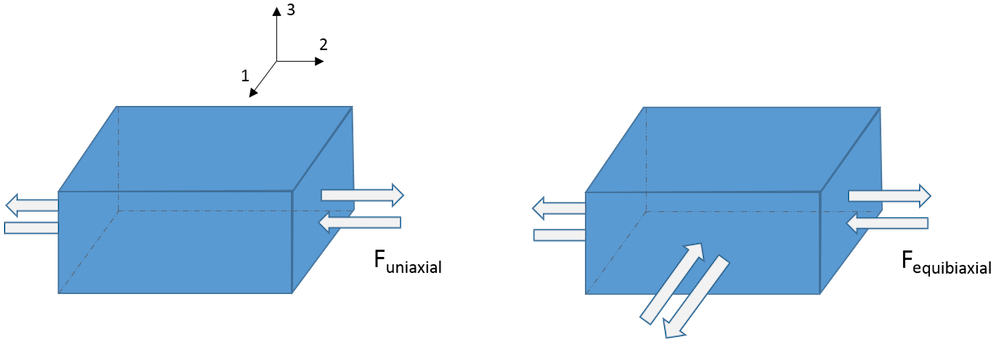
In a previous blog post on finding material data for structural mechanics simulations, we said that to correctly characterize a material deformation, it is crucial to have data from both uniaxial and equibiaxial tests. If we only have the uniaxial test data, then we get inaccurate results for simulating deformation states involving a multidimensional stress state.

The plot below shows a representation of the measured uniaxial and equibiaxial force-versus-stretch ratio \left(\lambda\right) for a foam material. A value of \lambda above 1 represents tension data, and a value of \lambda below 1 represents compression data.

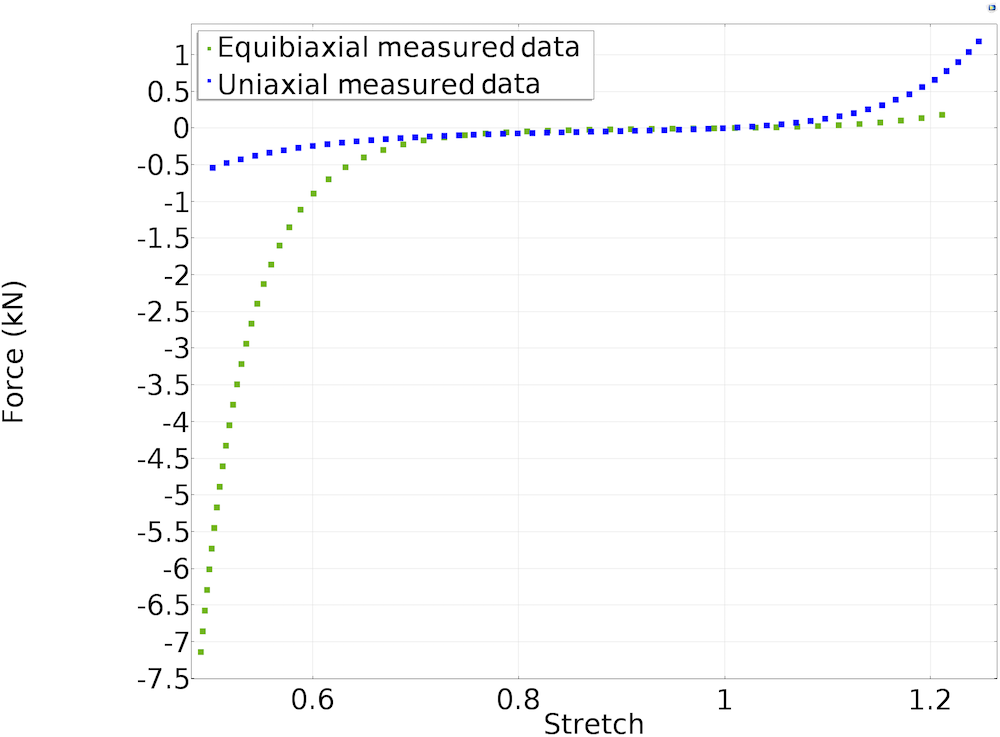
A representation of measured force-versus-stretch data for uniaxial and equibiaxial tests.

Storakers Material Model for Hyperelastic Materials

The Storakers material model is often used to model highly compressible foam. The strain energy density function for Storakers material model is given by

(1)

where \lambda_1, \lambda_2, and \lambda_3 are the principal stretches; J_{el} is the elastic volume ratio; and \alpha_k, \mu_k, and \beta_k are the Storakers material parameters.

In a hyperelastic simulation, the material parameters need to be provided as an input. These parameters are calculated by fitting experimental test data against analytical expressions representing stress or force versus stretch. We have discussed this general procedure in detail in a blog post on fitting measured data to hyperelastic material models. Unlike the incompressible material models we discussed in our previous blog post, we are investigating the analytic expressions for a compressible material in this blog post. Let’s take a look at the force-versus-stretch relationship for the Storakers material model corresponding to uniaxial and equibiaxial tests.

Uniaxial Tests

Referring to the schematic diagram above for a uniaxial test, let’s assume that the foam material used for material characterization is subjected to uniaxial loading in the principal direction 2. Assuming that only elastic deformation is admissible, the principal stretches for the uniaxial deformation of an isotropic hyperelastic material are given by

For uniaxial testing, the principal Cauchy stress in the principal directions 1 and 3 are given by \sigma_1 = \sigma_3 = 0. For compressible isotropic hyperelastic materials, the relationship between principal Cauchy stress and principal stretch is given by

(2)

The above relationship comes from one of the implications of the second law of thermodynamics and spectral representation of stress in terms of principal stretches. From the second law of thermodynamics, we have S = 2\frac{\partial W_s}{\partial C}, where S is the second Piola-Kirchhoff stress tensor and C is right Cauchy-Green tensor. In its spectral form S = \sum_{} _{a=1}^{a=3} \frac{1}{\lambda_a}\frac{\partial W_s}{\partial \lambda_a} \bf{\hat{N}_a} \otimes \bf{\hat{N}_a}, where \bf{\hat{N}}_a represents the principal referential directions.

Knowing that the Cauchy stress is \sigma = J^{-1}FSF^T and the spectral representation of deformation gradient tensor F is \sum_{} _{a=1}^{3} \lambda_a\;\bf{\hat{n}}_a \otimes \bf{\hat{N}}_a (and where \bf{\hat{n}}_a represents principal spatial directions), we can write \sigma = \sum_{} _{a=1}^{3} J^{-1}\lambda_a\frac{\partial W_s}{\partial \lambda_a}\; \bf{\hat{n}}_a \otimes \bf{\hat{n}}_a = \sum_{} _{a=1}^{3} \sigma_a\; \bf{\hat{n}}_a \otimes \bf{\hat{n}}_a, where \sigma_a are the principal Cauchy stresses. (Learn more about different stress measures and their directions here.)

Substituting the expression for W_s from Eq. 1 into \sigma_1, we get

However, it is also known that \partial J/\partial F = J F^{-\text{T}}, where J = \text{det}(F) and F is the deformation gradient tensor. This relationship comes from tensor calculus. When rewritten in terms of principal stretches, we have \partial J / \partial \lambda_i = J \lambda_i^{-1}. Substituting this relationship in the above equation and equating \sigma_1 to 0, we get

(3)

where the above equation holds for each \beta = \beta_k.

The uniaxial force is given by

(4)

where l_{1},l_{3} are deformed dimensions of the bar along the principal directions and l_{10}, l_{30} are the original dimensions of the bar along the principal directions. Using Equations 2 , 3, and 4, we can write the uniaxial force as

(5)

Equibiaxial Tests

Let’s assume that the foam material is subjected to equibiaxial forces in the principal directions 1 and 2 and only elastic deformation is admissible. For the equibiaxial deformation of an isotropic hyperelastic material, the principal stretches are

For equibiaxial testing, the principal Cauchy stress \sigma_3 = 0. Using Eq. 2, we get

(6)

where the above equation holds for each \beta = \beta_k.

The equibiaxial force F_{equibiaxial} is given by

(7)

Using Equations 2, 6, and 7, we get

(8)

Calculating Storakers Material Parameters with the Optimization Interface

Using the Optimization interface in the COMSOL Multiphysics® software, we perform curve fitting of the measured force-versus-stretch data against the analytical expressions derived in Equations 5 and 8 for N = 2. The plot below depicts the fitted data against the measured data. Equal weights are assigned to both the uniaxial and equibiaxial least-squares fitting.

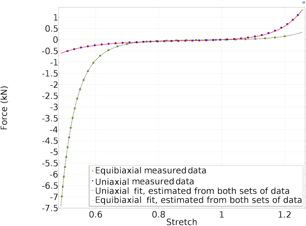
Fitted material parameters using the Storakers material model.

From the above fit, we calculate the Storakers material parameters for the tested foam material to be

Modeling the Compression of a Spherical Foam

Now that we have calculated the values of Storakers material parameters for the foam material, we can use these values directly in our simulation of the compression of the spherical foam. The figure below shows the setup for the simulation, where we have a hollow spherical foam being compressed by a smaller spherical indenter against a cylindrical rigid plate. The figure on the right shows the 2D axisymmetric representation of the 3D problem.

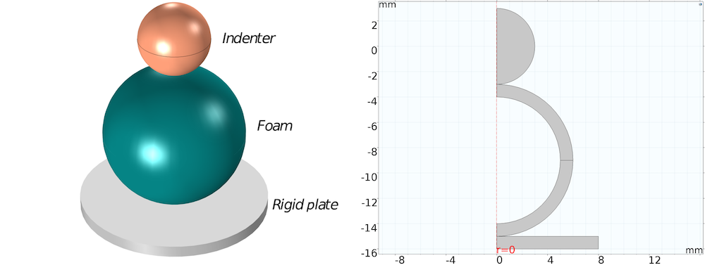
3D schematic of the compression of the foam material (left) and 2D axisymmetric setup in COMSOL Multiphysics (right).

The screenshot below shows the settings of the hyperelastic material model used for modeling the foam. The indenter and rigid plate are modeled as linear elastic materials.

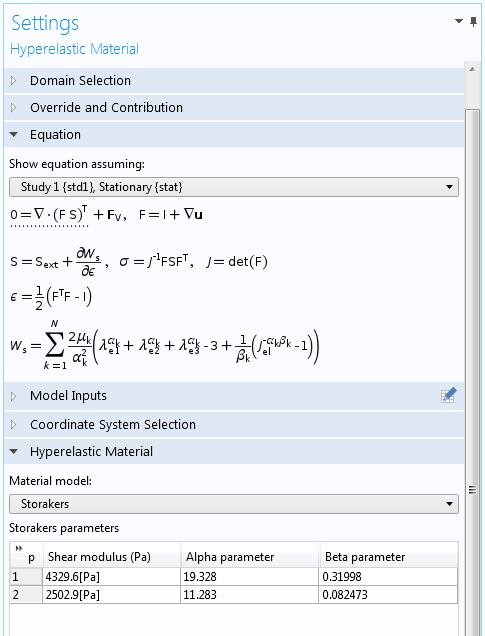
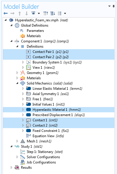
The indenter, foam, and rigid plate are in contact, so we define a contact pair between their boundaries. We allow the indenter to move downward by a total of 11 mm using a Prescribed Displacement condition. As a result, the inner foam boundary comes into contact with itself, known as self-contact.

We define a second contact pair to model self-contact, where we can define the inner boundaries of the foam as both source and destination — assuming that we don’t know what part of the inner surface will come into contact with what part of the same surface. The bottom rigid plate is set to be entirely fixed.

Settings for the hyperelastic material model.

Results and Concluding Remarks

The 3D animation below shows a plot of the von Mises stress in a section of the revolved geometry.

Von Mises stress in the spherical foam as it is compressed by the indenter. To see the variation in stresses throughout the animation, the maximum value of the color scale is capped at 10 kPa.

The plot below shows the contact pressure on the foam boundaries at the end of the simulation.

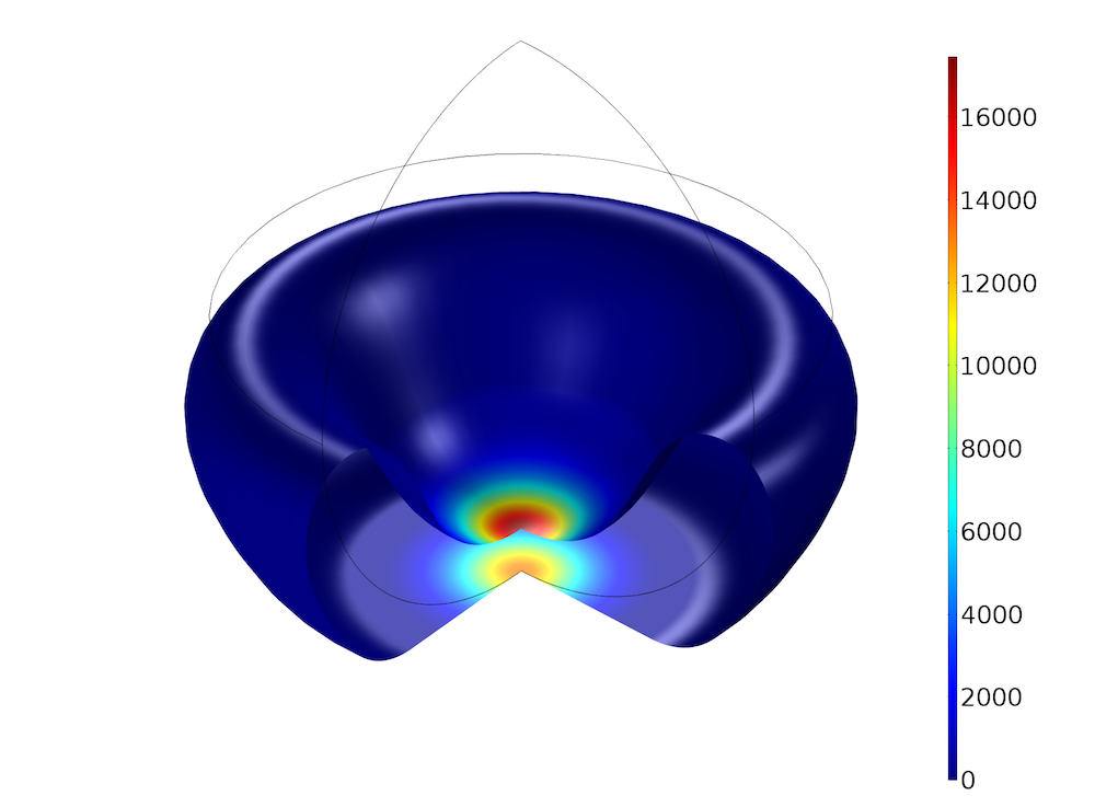
Plot of the contact pressure at the end of the simulation.

We are, of course, not limited to modeling a spherical foam. Now that we know the Storakers material parameters for a given range of stretch values, we can model the same foam in any other scenario, provided that its deformation is consistent with the test data used for calculating the parameters. We should also keep in mind, though, that despite obtaining the material parameters by curve fitting against experimental test data, the stability of the material model can still be problematic if the material model violates the Drucker’s stability criteria.

Next Step

Find out how the COMSOL® software can fit your structural analysis needs: