

Material models play an important role in describing, predicting, and understanding the physical behavior of a material. They describe the material response to external stimulations like force, heat, or voltage. Most material models are phenomenological in nature, based on experimental data and observations rather than underlying physical principles. A classic example is Hooke’s law, which governs linear elasticity and is widely used in various fields. Many simplifications and assumptions are necessary to make phenomenological material models computationally feasible, but this constrains their use for certain operating conditions. Hence, before using material models in real-world applications, it’s important to understand their responses in standard loading configurations. These configurations, known as standard material tests, serve as benchmarks for validation. In this blog post, we will look at how to test a numerical model in the COMSOL Multiphysics® software.
This is the second part in our blog series on working with numerical material models. In the first part of the series, we showed how to estimate the parameters of material models. Read Part 1 here.
Material Tests and the Test Material Feature
Some common types of material tests conducted in laboratories are explained in our blog post “Obtaining Material Data for Structural Mechanics from Measurements”. However, there are differences between testing a specific material and testing a numerical material model of it. As explained in the blog post, rubber is inherently elastic, but it becomes as brittle as glass when submerged in liquid nitrogen. Conversely, glass, which is naturally brittle, becomes viscoelastic when heated. Hence, one material may require different material models under varying operating conditions to describe its behavior accurately. When a specific material is tested in a laboratory, numerous factors affect the test results, such as the size and geometry of the specimen, applied loads, boundary conditions, operating conditions, and time dependency. However, numerical testing of a specific material model is often simpler, with fewer operating parameters being used.
Most material models are phenomenological in nature, and they are mathematical approximations of a true physical behavior. These models are based on the experimental measurements obtained through different standard tests. Although phenomenological models are not derived from the laws of physics, these laws, nevertheless, enforce limits on the mathematical structure of material models and the possible values of material properties. It’s thus important that material properties, even for well-established material models, are chosen wisely and that their responses to different standard tests are evaluated. Apart from this, there are other reasons to test a numerical material model using different tests, such as to:
- Evaluate correctness of the material properties by comparing the numerical results with experimental results
- Find the valid stress and strain range before performing the numerical simulation
- Check the direction dependency of stress and strain components
- Check the presence of material instabilities, such as limit point instability
Version 6.1 of the COMSOL Multiphysics software introduced a new feature in the Solid Mechanics interface called Test Material, which enables testing different material models using a set of standard tests. The different material tests available with the Test Material feature include the:
- Uniaxial test
- Biaxial test
- Shear test
- Isotropic test
- Oedometer test
- Triaxial test
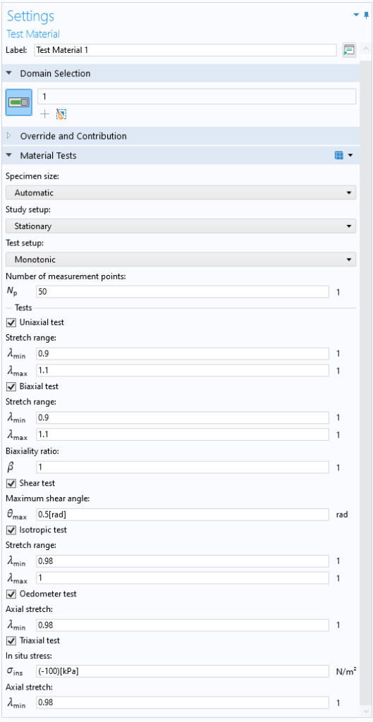
Settings for the Test Material feature with the Monotonic option selected as the test setup.
The domain selection in the feature settings determines which material model will be tested. Users can always change the domain selection of a Test Material feature or use multiple Test Material features to test multiple material models. The feature includes an action button folder called Automated Model Setup in the Material Tests section of the feature. This button folder includes buttons for setting up and removing the tests. Clicking the Set up Tests button results in the following actions:
- A new 3D component is created.
- A geometry of a 3D block of predefined size is created. Its size is defined by Specimen size; the default is a 1-meter-sized block.
- A new Solid Mechanics interface is added to this component. The displacement discretization is set to linear.
- Boundary conditions and loads that correspond to the selected tests are added to the new Solid Mechanics interface.
- A mesh node with a single element is created.
- A new stationary or time-dependent study node is added.
- A stop condition is added to the stationary or time-dependent study. This condition stops the loading when the element is fully collapsed.
- A set of default plots is added to the Results node.
Note that the specimen size influences some material models. In such cases, the size of the 3D block needs to be changed, which can be done by choosing the user-defined option in the Specimen size list.
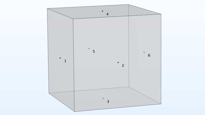
The geometry used for different tests. The numbers indicate the selection numbers of boundaries in COMSOL Multiphysics.
The material tests can be either stationary or time dependent. The transient tests are important for testing time-dependent material models like creep, viscoelasticity, etc. The choice of study type can be decided with the Study setup list. When the time-dependent option is chosen, an extra input for the test time will appear in the user interface (UI). Apart from the Study setup list, the Test setup list also defines the setup of material tests. The options for this include:
- Monotonic: For material models without hysteresis and dissipation effects, monotonic tests are enough to describe their behavior. Common examples of such material models include elastic materials, where loading and unloading of the material give the same stress–strain response. With the Monotonic option, you can change the number of measurement points for the selected material tests. All six material tests are available with this option.
- Cyclic: For material models incorporating inelastic effects, hysteresis and dissipation are inherent in nature. Their loading and unloading responses are different. For such material models, it’s necessary to perform cyclic material tests. Any elastoplastic material can fit into this category. With the Cyclic option, apart from adjusting the number of measurement points, you can adjust the number of cycles. Only uniaxial and isotropic tests are available with this option.
- User defined: As the name suggests, you can run material tests with the help of a function written in terms of principal stretches or forces. This option provides more flexibility than the first two options. With a stationary study, an auxiliary parameter is needed as an independent parameter for a function, while the time acts as an independent parameter for a function in time-dependent studies. Only uniaxial, biaxial, and isotropic tests are available with this option.
In the next section of this blog post, we discuss the setup of each material test option.
The Material Test Options
Uniaxial Test
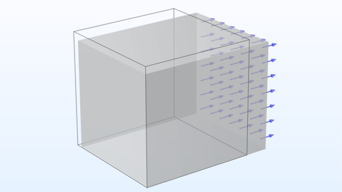
Test schematic: the prescribed normal displacement of boundary 6; the normal displacements of boundaries 1, 2, and 3 are constrained.
The tensile tests are most commonly used when working with metals. Many material properties like Young’s modulus, Poisson’s ratio, yield strength, etc., can be obtained by using this type of test. For some materials that have little capacity to carry tensile loads (e.g., concrete), the uniaxial compression test is preferred over the uniaxial tensile test. With help of the Test Material feature, a uniaxial tensile or compression test can be used to obtain the uniaxial stress–strain relation, strain hardening for elastoplastic models, hysteresis in the material, etc. To run a uniaxial test using the Test Material feature, a stretch range must be given. The minimum stretch, \lambda_\textrm{min}, gives the compressive limit, and the maximum stretch, \lambda_\textrm{max}, gives the tensile limit. A uniaxial compression test is achieved by setting \lambda_\textrm{max} = 1, and a uniaxial tension test is achieved by setting \lambda_\textrm{min} = 1. The inputs must have the relation \lambda_\textrm{min} < \lambda_\textrm{max}.
The blog post mentioned earlier, “Obtaining Material Data for Structural Mechanics from Measurements”, includes an animation illustrating uniaxial tension and compression tests for three different material models: a linear elastic material, an elastoplastic material with isotropic hardening, and an elastoplastic material with kinematic hardening. Similar results can easily be generated using the Test Material feature. The Test Material feature automatizes the model setup needed to run different material tests and presents important results as default plots. This streamlines the entire material testing process for users, enabling them to perform the action with just one click rather than having to set up the model manually.
Once the results of the material tests are evaluated, the autogenerated nodes in the Model Builder tree can easily be removed using the Remove Tests button of the Test Material feature. This ensures that users can transition to the main simulation once the required tests are performed for the chosen material model.
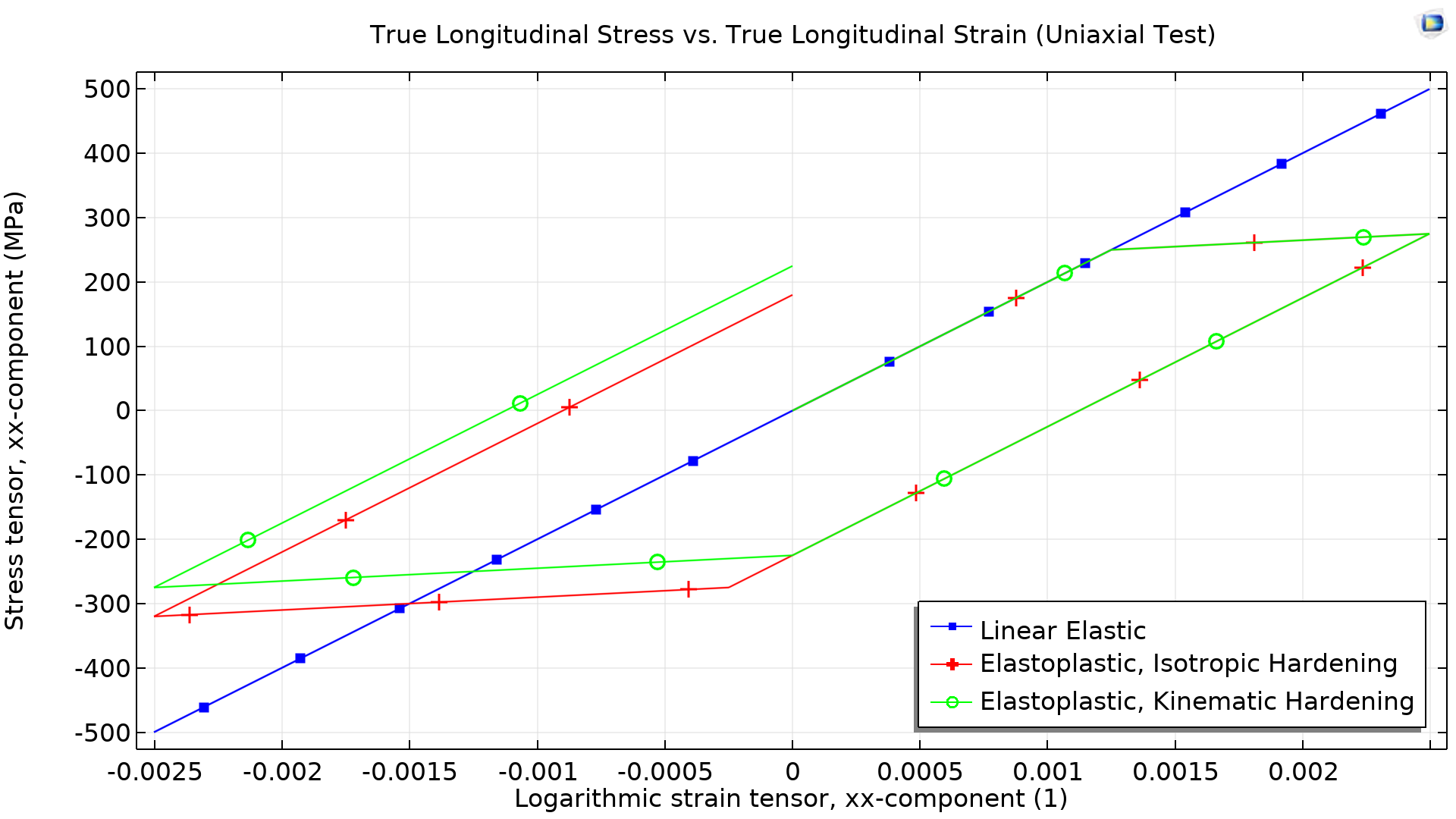 The stress–strain response from uniaxial tension and compression tests for different material models using the Test Material feature.
Let’s now go over the importance of numerical material model testing for a more intricate constitutive law. Ref. 1 presents a nine-parameters Mooney–Rivlin (MR) material model, augmented with additional strain-rate-dependent terms, specifically tailored for a polyurea elastomer. The generalized, nearly incompressible MR material is characterized by a strain energy density function expressed as:
For a nine-parameter Mooney–Rivlin material, m= 3, n= 1, and C_{00} = C_{13} = C_{31} = C_{23} = C_{32} = C_{33} = 0. Ref. 1 proposes a modified strain energy density dependent on strain rate:
Here, \mu is the strain rate parameter, \dot{\epsilon} is a true strain rate, and \dot{\epsilon}_\textrm{ref} is a reference strain rate. The material properties determined from the tensile test experiments are:
| C_{10} \mathrm{(MPa)} | C_{01} \mathrm{(MPa)} | C_{20} \mathrm{(MPa)} | C_{02} \mathrm{(MPa)} | C_{11} \mathrm{(MPa)} | C_{30} \mathrm{(MPa)} | C_{03} \mathrm{(MPa)} | C_{12} \mathrm{(MPa)} | C_{21} \mathrm{(MPa)} | \kappa \;\mathrm{(MPa)} | \mu |
|---|---|---|---|---|---|---|---|---|---|---|
| 203 | -185 | 28,146 | 27,379 | -55,745 | 3264 | -7800 | 14,219 | -14,283 | 3600 | 0.17 |
The modification proposed by the authors in Ref. 1 adds a multiplier factor to the original MR strain energy density function. Their first loading case considers \dot{\epsilon} = \dot{\epsilon}_\textrm{ref} = 0.02/s, which reduces the modified strain energy density to the original MR strain energy density. This case is considered here to run uniaxial tension and compression tests using the Test Material feature. The results of the uniaxial tension test exhibit qualitative consistency with those reported in Ref. 1; some small differences between the values are expected due to the different specimen used for the numerical simulations. Nevertheless, the results of the uniaxial compression test are nonphysical, as the uniaxial stress turns positive for compressive strain after a certain level of compression. Also, a simulation will fail as soon as the stress versus strain curve gets a nonpositive slope. This clearly displays the risk of applying curve-fitted material models outside the range of strains states at which the measurements were made. In this case, the material model is valid only for tension. So, if you have a set of material parameters for which you are uncertain about the origins, checking the response under different relevant strain states is more or less necessary.
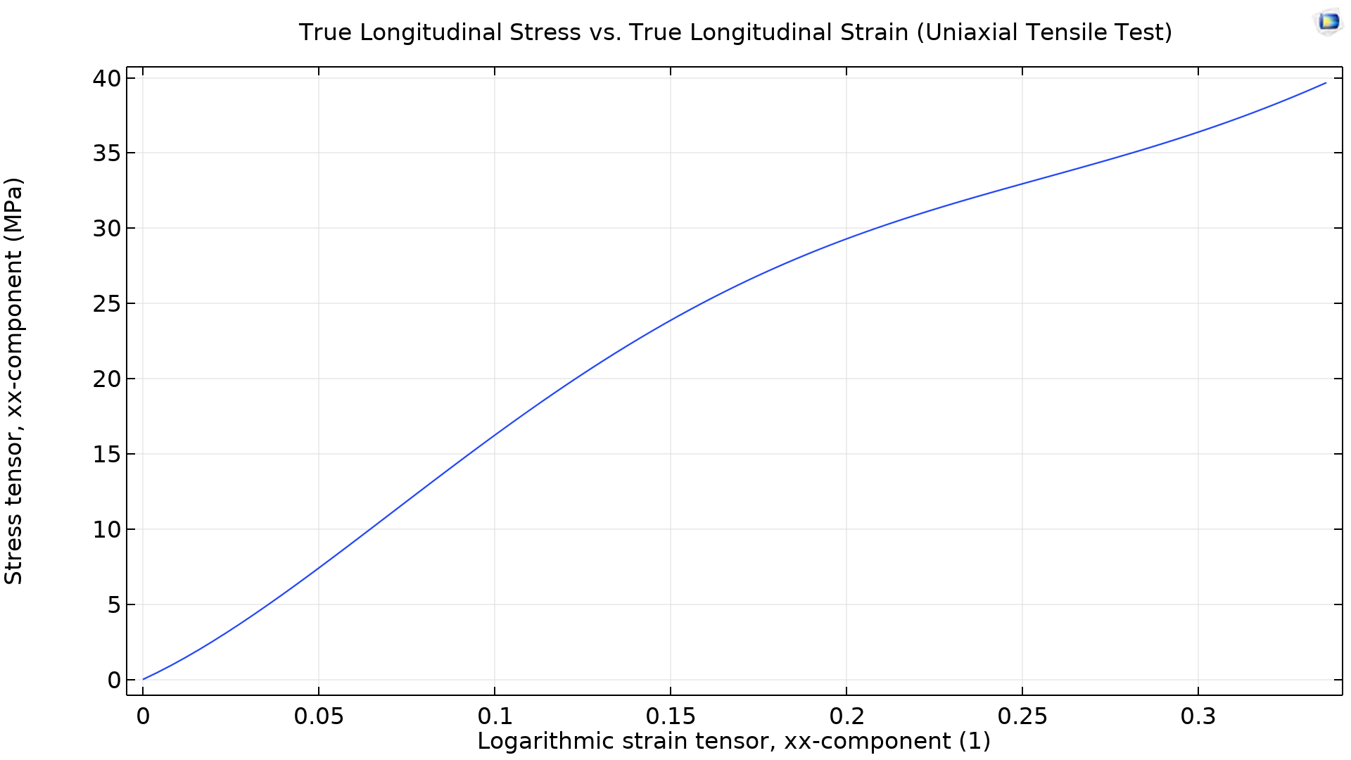
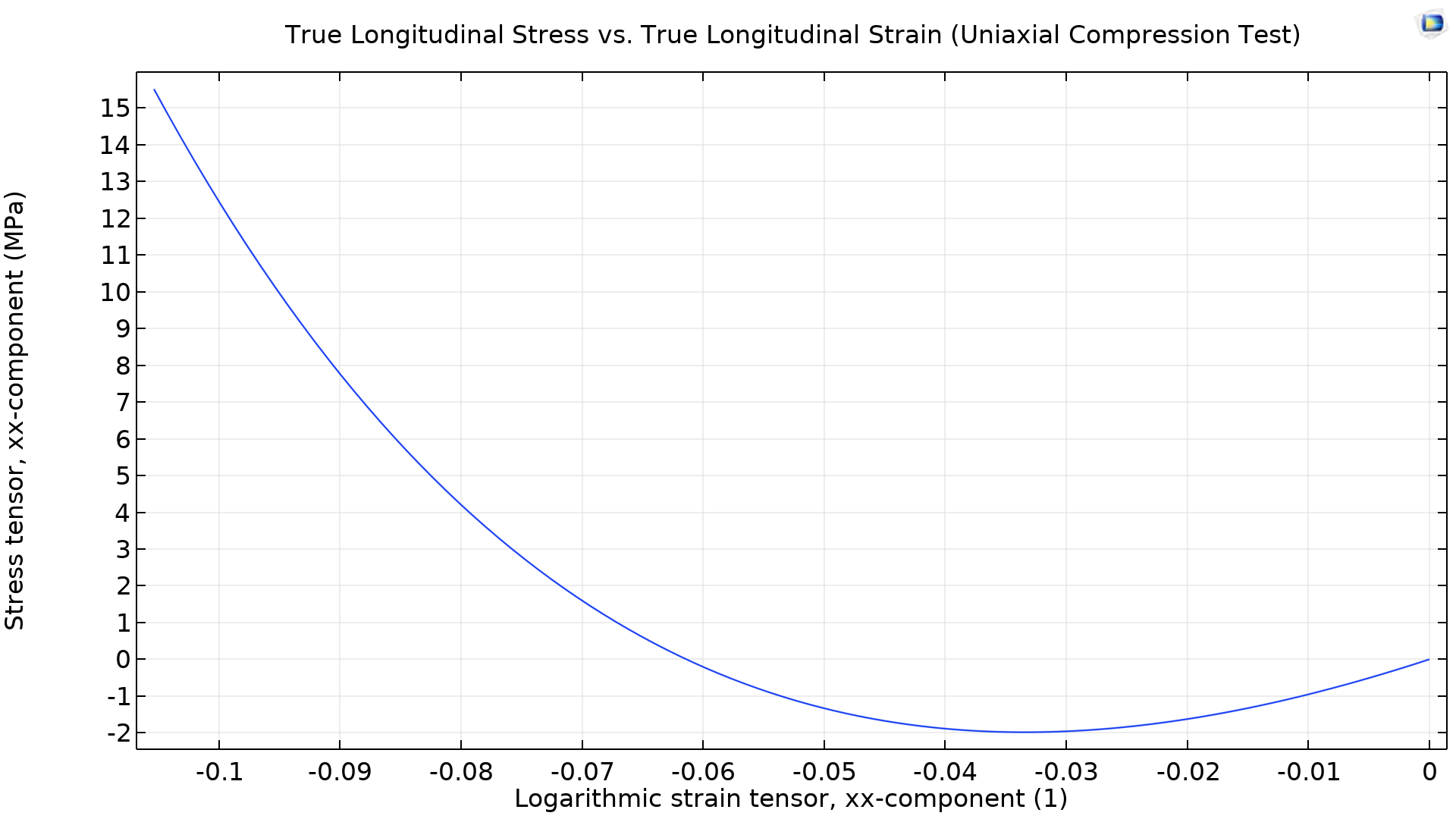
The left- and right-hand images show the stress–strain response from uniaxial tension and compression tests, respectively.
The Concrete Damage–Plasticity Material Tests example in the Application Libraries uses the Test Material feature to observe the response of a coupled damage–plasticity concrete model for different loading conditions. In this example, three uniaxial tests are conducted:
- Uniaxial monotonic tension and compression
- Uniaxial cyclic loading (tension to compression to tension)
- Uniaxial cyclic loading (compression to tension)

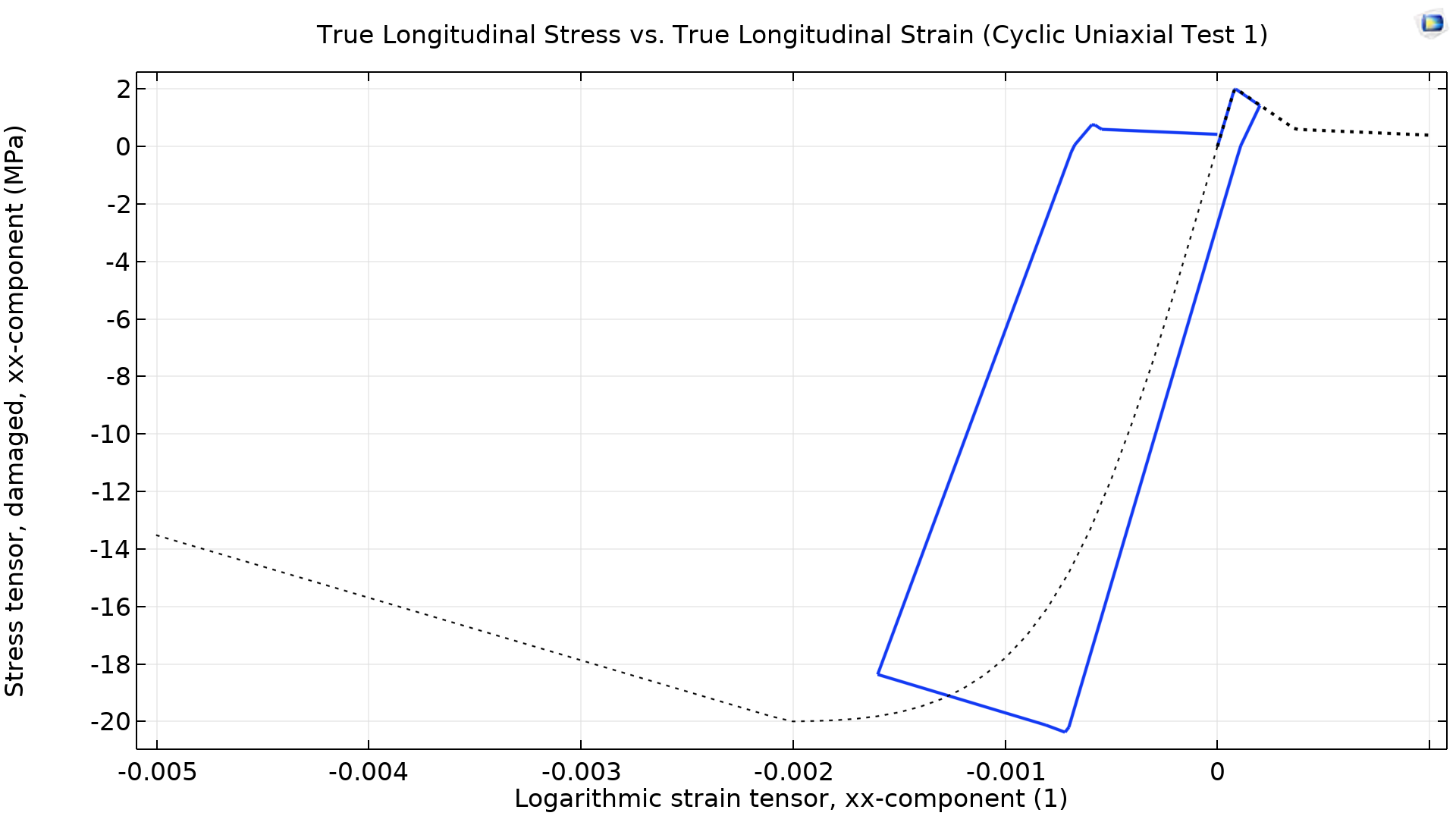
Left: The stress–strain response from uniaxial monotonic tension and compression tests. Right: The stress–strain response from a uniaxial cyclic loading test (tension to compression to tension). The dotted black curve shows the stress–strain response of a monotonic uniaxial test.
The results of the uniaxial monotonic tension and compression tests show the characteristic dissimilarity of concrete in compression in comparison with tension. The results from the cyclic tests show a big difference when compared to the monotonic test due to irreversible deformation. All available plastic deformation in the cyclic test occurs when the specimen is loaded in tension and starts to crack. Hence, there is no plastic hardening when the stress is reversed to compression; instead, the response is elastic until softening starts.
Biaxial Test

Test schematic: the prescribed normal displacements of boundaries 5 and 6; the normal displacements of boundaries 1, 2, and 3 are constrained.
For anisotropic materials, the stress–strain relation becomes complicated, and to characterize the constitutive law, you must account for the multiaxiality of stresses and strains. The biaxial test creates a state of multiaxial loading, which allows the evaluation of material response under combined tensile, compressive, and shear stresses. Just like with a uniaxial test, the biaxial test needs \lambda_\textrm{min} and \lambda_\textrm{max} user inputs. In addition, the biaxial test needs a biaxiality ratio, \beta. The biaxiality ratio determines the magnitude of the load in the second principal direction.
The Concrete Damage–Plasticity Material Tests example uses the Test Material feature to run a monotonic biaxial compression test. The stress in one principal direction shows a different relationship with respect to the strains in three principal directions, which gives more insight than the results of the uniaxial test discussed previously.
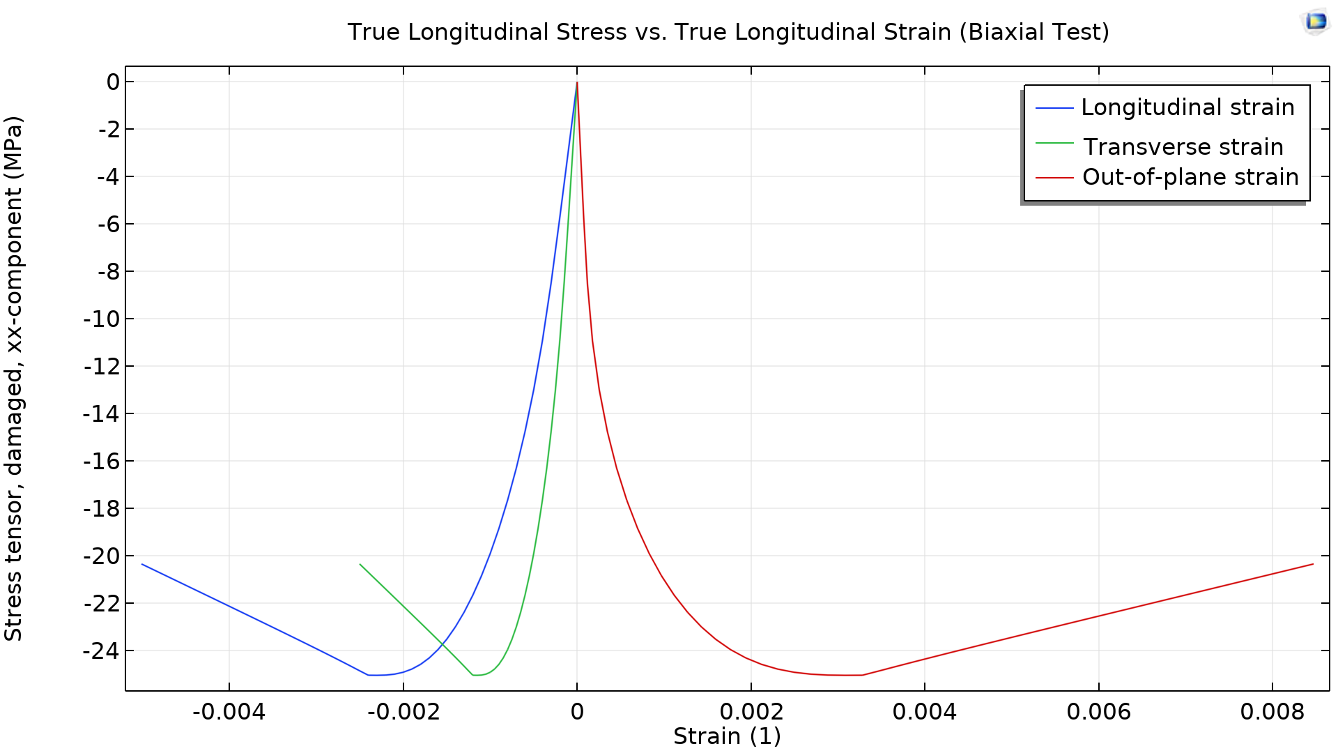 The stress–strain response from a biaxial monotonic compression test.
The Primary Creep Under Nonconstant Load example in the Application Libraries shows how to use the Test Material feature to evaluate creep behavior of material under nonconstant uniaxial and biaxial loading. For the Norton creep model, analytical formulas are available, so the Test Material feature can be used to set up tests and compare the numerical results with analytical or experimental ones.
Shear Test
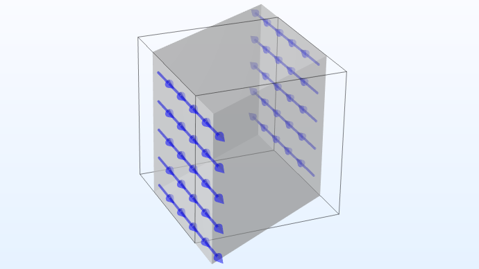
Test schematic: the prescribed tangential displacements of boundaries 1 and 6; the normal displacements of boundaries 1, 3, and 6 are constrained.
Shear tests are important for understanding a material’s response to shear loading and for determining material properties such as shear modulus. While many materials respond well to tension and compression loading, they may not perform well under shear loading due to internal sliding or slippage of material layers. In applications where shear loads are predominant, it’s necessary to assess the material’s response to such loads before using it. The Test Material feature has a single user input for the maximum shear angle, \theta_\textrm{max}, to conduct a simple shear test.
In “Estimating Hyperelastic Material Parameters via a Lap Joint Shear Test”, a guest blog post on the COMSOL Blog, a simple lap joint shear test is discussed. In the blog post, experimental results obtained from the lap joint shear test are used to get the material properties of a Yeoh hyperelastic material model based on a curve-fitting approach. The strain energy density for a nearly incompressible Yeoh material is written as
where \bar{I}_1 is the first isochoric invariant of the elastic right Cauchy–Green deformation tensor, and J_\textrm{el} is the elastic volume ratio. The material properties obtained after optimization can be found in the table below.
| Material Properties | Value (MPa) |
|---|---|
| c_1 | 0.656 |
| c_2 | 0.034 |
| c_1 | -0.00072 |
| \kappa | 656 |
For the purpose of this blog post, the results presented in the guest blog post are reproduced and presented here (see the graphs below).
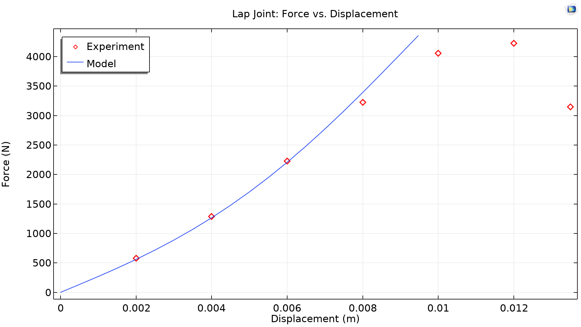
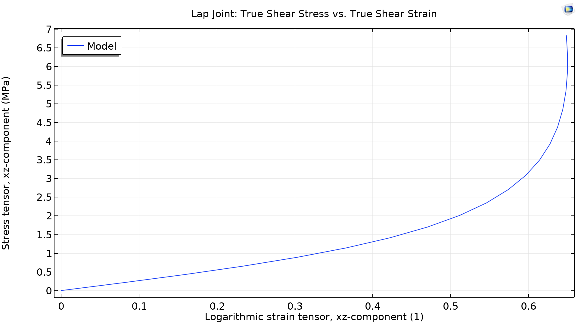
Left: The force-displacement curves from the experimental results and the numerical simulation of the lap joint test. Right: The shear stress–shear strain curve based on an average over the domain from the numerical simulation of the lap joint test.
In this blog post, we will use the constitutive law and material properties from the aforementioned blog post and conduct a simple shear test using the Test Material feature. The shear stress–shear strain response curve obtained from the Test Material feature is very close to the curve obtained from the actual lap joint test above. The specimen in the actual lap joint test is designed to, as closely as possible, induce homogeneous pure shear. This makes it possible to compare with the response from the Test Material feature.
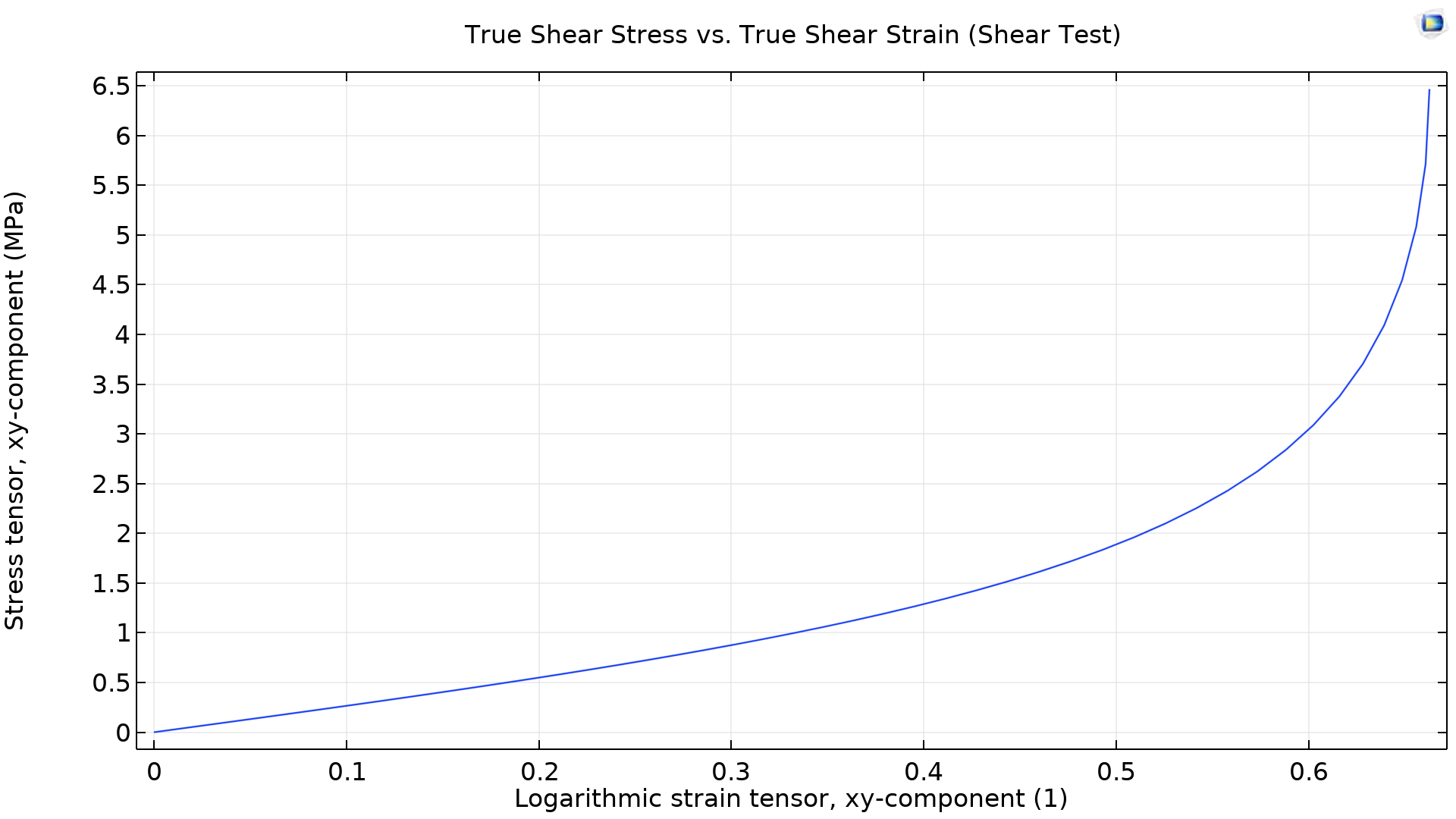 The shear stress–shear strain response from a shear test run with the Test Material feature.
Isotropic Test
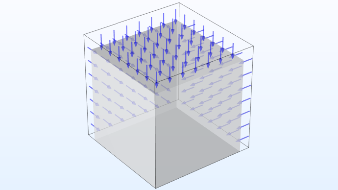
Test schematic: the prescribed normal displacements of boundaries 4, 5, and 6; the normal displacements of boundaries 1, 2, and 3 are constrained.
The constitutive laws of soils, concrete, and rocks are nonlinear and elastoplastic in nature. Unlike metals, plasticity in soils cannot be classified as J2 plasticity due to its dependence on the hydrostatic pressure. The isotropic compression test is a fundamental test in soil mechanics, as soils cannot sustain tension. It can be used to understand a soil’s response to triaxial compression. Just like with the uniaxial test, the isotropic test needs \lambda_\textrm{min} and \lambda_\textrm{max} user inputs in the Test Material feature.
The Isotropic Compression with Modified Cam-Clay Material Model example in the Application Libraries shows use of the Test Material feature to generate an isotropic compression response of a modified Cam-clay material model. The relation between the void ratio and the logarithm of the pressure can be recovered from the test, which is a fundamental relation for this constitutive law.
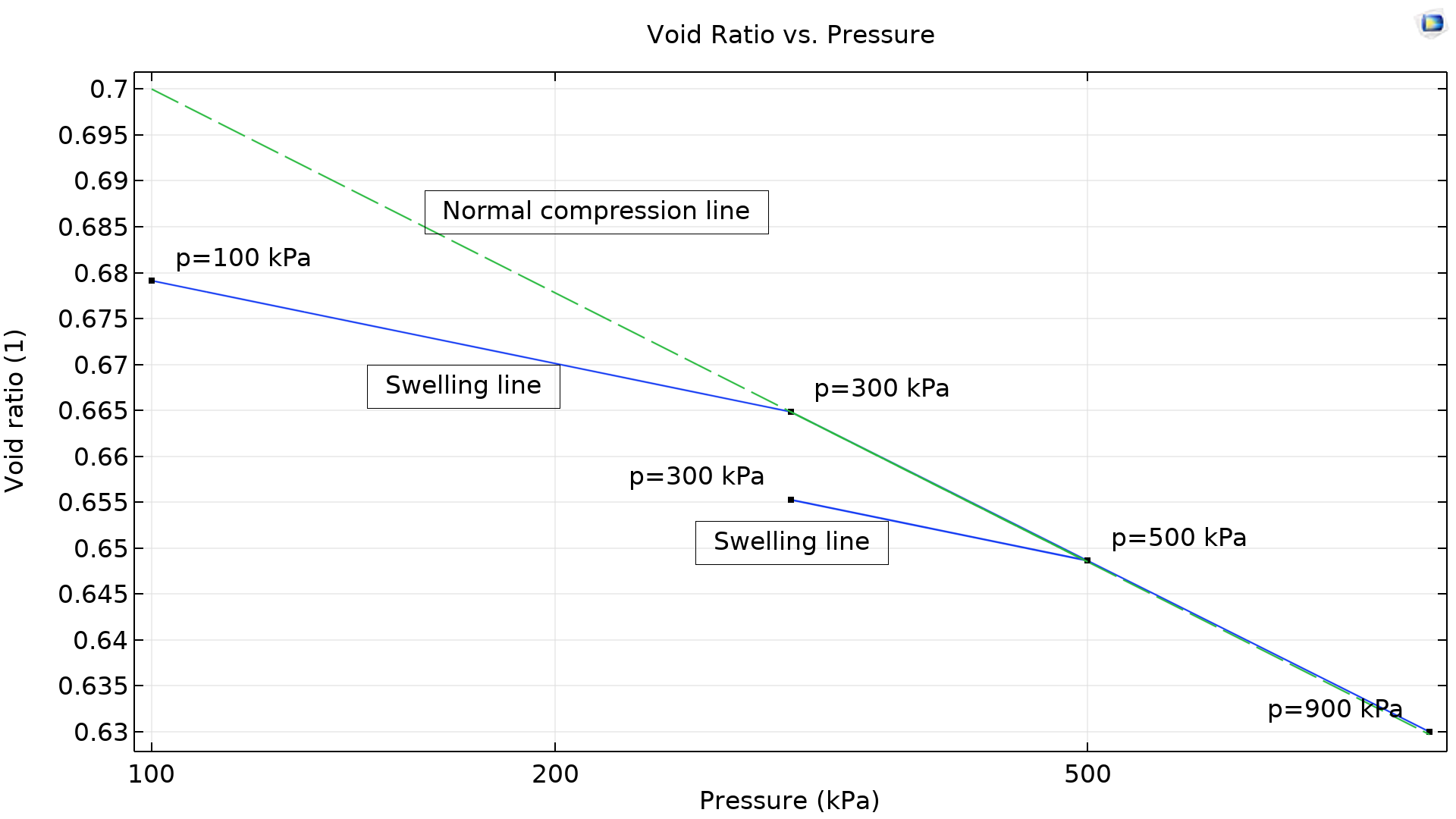 The void ratio–pressure response from an isotropic test.
Oedometer Test
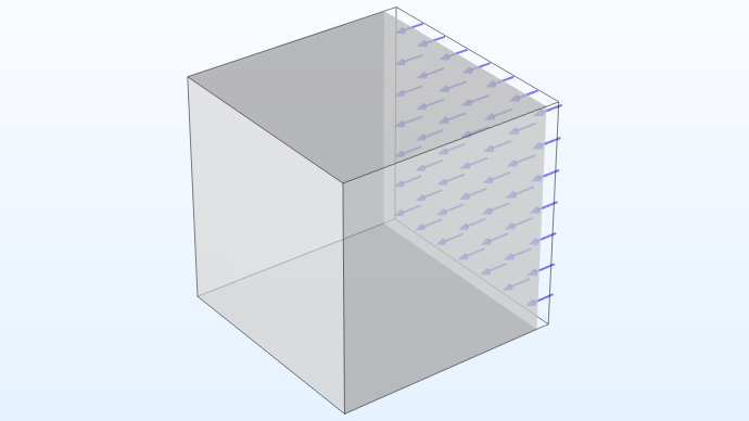
Test schematic: the prescribed normal displacement of boundary 6; the normal displacements of all other boundaries are constrained.
The oedometer test is a special type of uniaxial test wherein one boundary is either extended or compressed while constraining other boundaries. This test is also known as a consolidation test in soil mechanics and is used to determine the consolidation characteristics of soils under vertical loads. There is only one user input, \lambda_\textrm{min}, in the Test Material feature to drive this test.
Triaxial Test
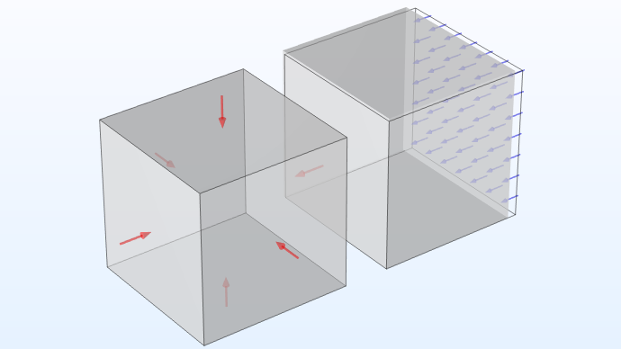
Test schematic: isotropic compression in the first step. In the second step, normal displacement is prescribed on boundary 6; the normal displacements of boundaries 1, 2, and 3 are constrained.
The triaxial test is extensively used to determine the physical properties, stress–strain response, and failure criterion of soils and rock materials under multiaxial stress conditions. As stated previously, the plasticity models of soils depend on shear stress as well as mean stress; hence, triaxial tests are important for understanding their behavior. The triaxial test consists of two steps: The first step is isotropic compression, and the second step is uniaxial compression. The first step consolidates the soils, and depending on the consolidation, the subsequent stress path changes due to shear stress created by the second step. The Test Material feature has two inputs for the triaxial test: first is In situ stress, \sigma_\textrm{ins}, and second is Axial stretch, \lambda_\textrm{min}.
Our blog post “Analyzing Triaxial Testing Methods for Geomechanics” discusses the triaxial test and its importance in geomechanics. The Triaxial Test example in the Application Libraries sets up a triaxial test in a detailed manner. In this example, a linear elastic material with a Drucker–Prager plasticity material model is tested. If the triaxial test is run with the Test Material feature in the existing setup, the results will match that presented in the example. The Test Material feature presents a quick and easy alternative to the existing detailed model setup.
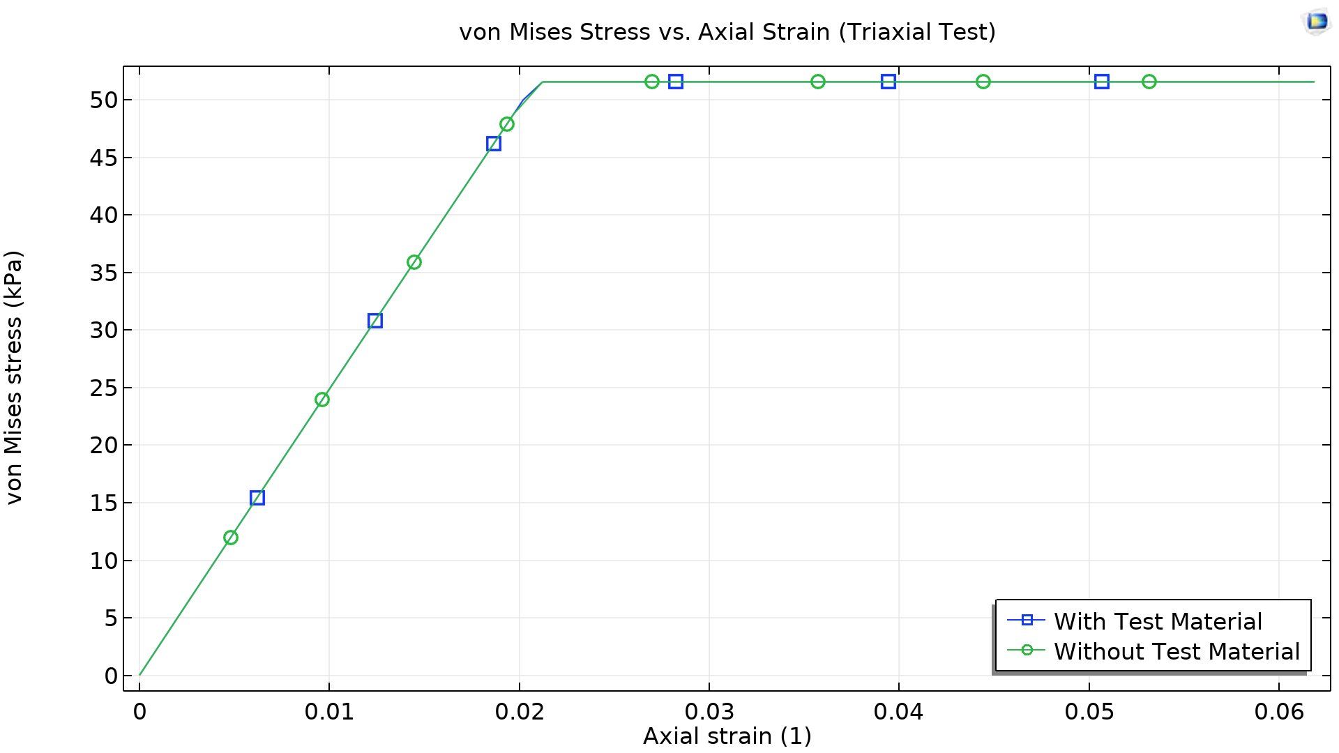 The von Mises stress–axial strain response from a triaxial test.
Note that the schematics and description here are presented considering user inputs in terms of stretch ranges. However, when the Test setup is set to User Defined, an addition user input, Test control, appears. When Test control is set to force-driven, user inputs can be specified in terms of pressure.
Summary
Numerical material models need to be evaluated and tested through simple material tests before being used in large-scale simulation. The Test Material feature serves as a valuable and convenient tool for this purpose. With the Test Material feature, it’s easy to set up multiple tests, evaluate the material response, and, if not needed, clear the autogenerated model nodes.
Reference
- D. Mohotti et al., “Strain rate dependent constitutive model for predicting the material behaviour of polyurea under high strain rate tensile loading,” Materials & Design, vol. 53, pp. 830–837, 2014.
Further Learning
To learn more about material models and testing, check out these blog posts:


Comments (0)