How to Use Interpolated Material Data to Model Irregular Geometries

We have already discussed different ways to create geometry objects of irregular shapes on the blog. In this blog post, we will demonstrate an incredibly powerful alternative approach by using interpolation functions. Instead of creating geometry objects, we will indirectly define the irregular shape by taking advantage of the spatial variation of a material property in the object we want to study.

What If I Can’t Create an Irregular Geometry?

Say that, by some measurement technique, we have been able to obtain data that describes how a material property varies inside a representative volume of a material. By visualizing the data, we can identify several regions with distinct properties; for example, the pores and the solid regions in a block of porous material. But what do we do if the identified regions form highly irregular shapes that are not suitable for generating geometry in the COMSOL Multiphysics® software?

If we have access to the material properties in coordinates inside our representative volume, the shape of which we can easily draw, then we can use an interpolation function based on this data to define the material for our simulation, thus skipping the creation of the irregularly shaped geometry object altogether.

One example is in the Pore-Scale Flow tutorial model, where we solve the incompressible, stationary Brinkman equations on a rectangular-shaped domain with material parameters based on an image function.

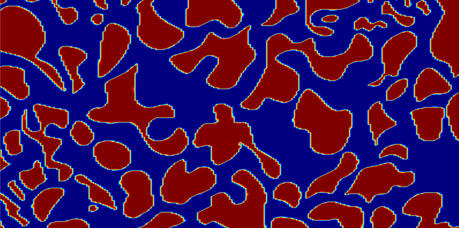
The image function representing the porous medium used in the Pore-Scale Flow tutorial. The color ranges from 0 to 1, where blue (0) represents the fluid and red (1) the solid.

In the regions marked with red, the material parameters are set to imitate a solid, and the material parameters for the fluid are defined in the blue region.

An Irregular Shape Made Regular: RF Simulation of a Human Head

Let’s return to the previously discussed model of the human head, which we lofted based on curve data in different cross sections. Say we don’t have the curve data needed to loft the head or access to the Loft operation in the add-on Design Module. Instead, we have a text file with the material properties defined in coordinates inside the region. Let’s start by introducing the tutorial where the geometry of the head is used.

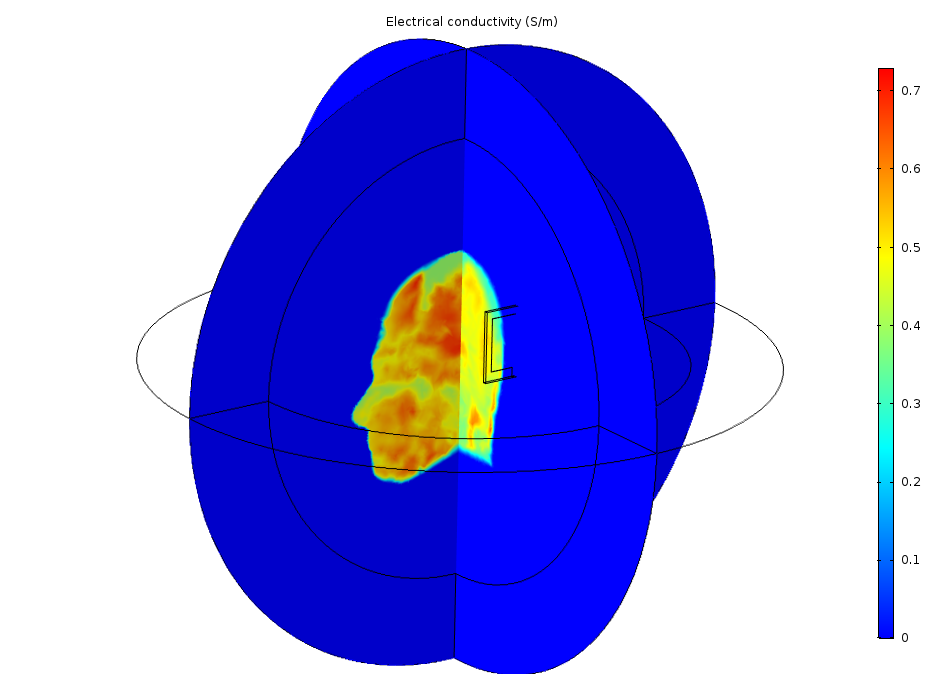
Slice plot showing the electrical conductivity (S/m) for the air (dark blue) and the head.

The Specific Absorption Rate (SAR) in the Human Brain tutorial models the absorption of a radiated wave from an antenna into a human head, as well as the resulting increase in temperature. The patch antenna is placed on the left side of the head and is excited by a lumped port. The tutorial described in this blog post demonstrates how to set up the model without the geometry of the head and shows what modifications are needed to accomplish this.

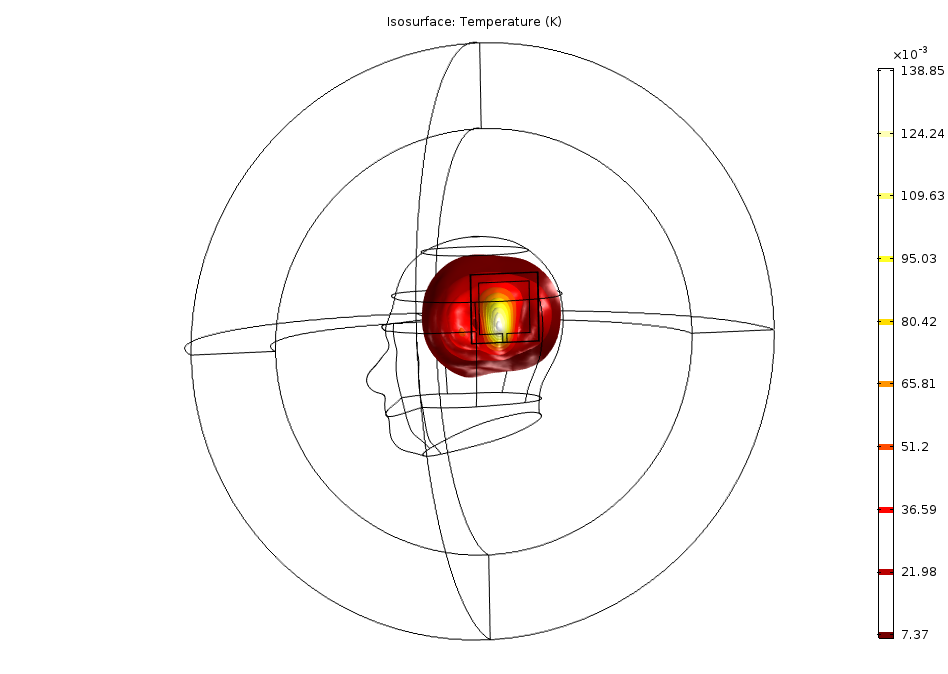
Specific Absorption Rate (SAR) in the Human Brain tutorial model. The isosurfaces show the temperature increase, dT (K), as a result of the absorbed radiation from the antenna.

The goal is to import material data into interpolation functions that we can use to define the material properties for the computational domain, which will become much simpler. Without the head geometry, we only need the sphere, which represents both the head and surrounding air, and the domains for the perfectly matched layers (PMLs). We also keep the smaller block with added edges, which represents the patch antenna.

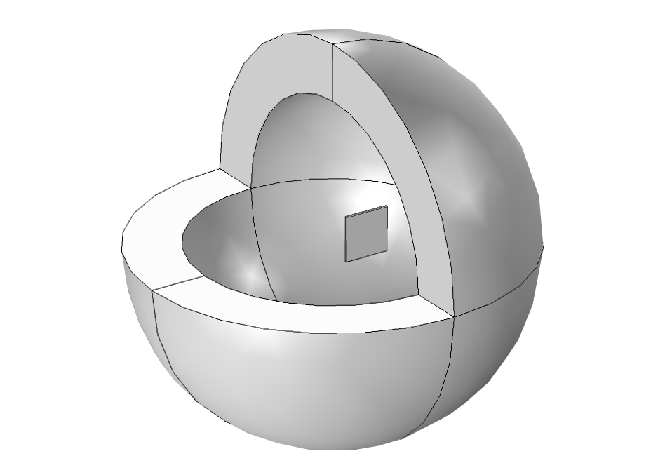
Geometry for the simulation without the geometry object for the head.

Using a Text File to Create Interpolation Functions in COMSOL Multiphysics®

A text file with material data can be formatted in different ways. For this example, the Spreadsheet format is used. In such a text file, there is one column each for x-, y-, and z-coordinates followed by an arbitrary number of data columns. The columns in the text file of our model include:

• Space dimensions: x, y, z
• Thermal conductivity: k (W/(m*K))
• Relative permittivity: epsr (1)
• Relative permeability: mur (1)
• Electrical conductivity: sigma (S/m)
• Blood perfusion rate: omega_head (1/s)

If the text file contains NaN entries, it is usually recommended to replace them with zero, a large value, or a small value, depending on the material property, as it triggers solver errors if the functions interpolate to NaN in the calculation domains. We create one Interpolation function per data column in the file and add the units for the arguments as well as the function itself so that the units are correctly recognized in the physics. When all data columns have the same unit, it is possible to create all functions within the same Interpolation feature.

We create the Interpolation features in the Global Definitions section of the Model Builder, since we want the material property functions not only for defining the material properties for the physics but also for helping generate a finer mesh where the surface of the head would be. To do this, we use a Size Expression feature when generating the mesh, as discussed later in the blog post.

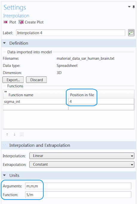
The Settings window for one of the interpolation functions. The number in the Position in file field corresponds to the number of the data column, starting from 1. In this image, sigma_int is taken from the fourth data column in the text file. The unit of the function can be entered in the bottom of the Settings window.

Creating Variables to Identify Locations Inside and on the Head

When geometry boundaries define the transition from one domain to the next, the mesh must always follow the shape of the faces that separate the domains. Here, there are no faces that represent the head, so we need to manually tell the mesh algorithm where it is important to refine the mesh. The mesh size can be about the same inside the head as outside the head, so it is most important to resolve the border between the two materials (head and air). In general, it is important to resolve a change between materials as that will typically impose a gradient in the fields. The larger the gradients, the finer the mesh must be to resolve the transition. For some applications, it is important to also resolve the mesh in the complete domain and not just at the borders between the different materials.

To refine the mesh along the shape of the head, we add two global variables based on the interpolation function k_int, as that function is 0.5 W/(m*K) and almost zero in the air. The variable avMat is 1 inside the head and onBnd is 1 in the vicinity of the boundary:

avMat = (k_int(x-d,y,z)/0.5+k_int(x+d,y,z)/0.5+k_int(x,y-d,z)/0.5+k_int(x,y+d,z)/0.5+k_int(x,y,z-d)/0.5+k_int(x,y,z+d)/0.5)/6

onBnd = (avMat>0.01)*(avMat<0.99)

The parameter d is equal to the fine mesh size that is used in the Size Expression node and defines the thickness of the area where the mesh is refined (highlighted in red in the following image).

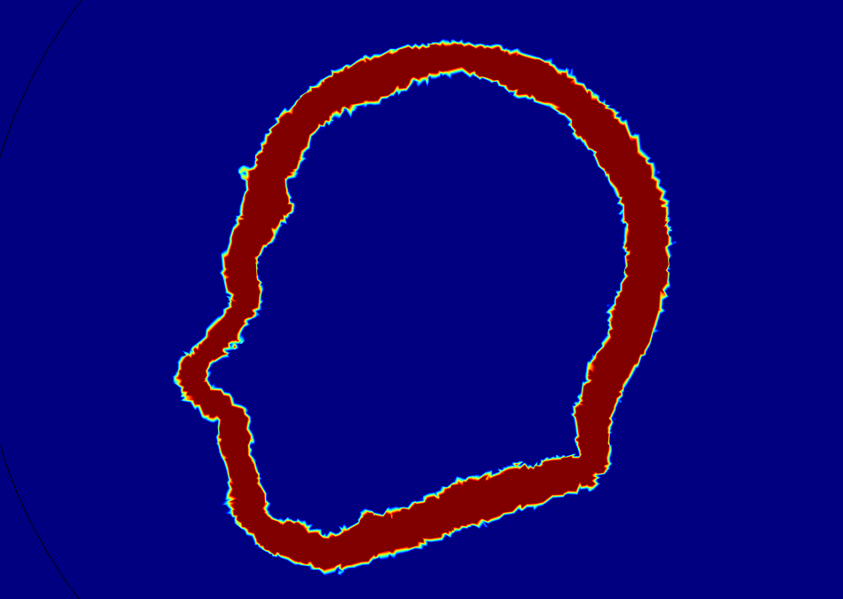
A slice plot of the onBnd variable. The values range from zero (blue) to 1 (red). The mesh is refined in the region shown in red using a mesh Size Expression.

Building a Finer Mesh to Resolve the Head Shape

Under the Free Tetrahedral node in the Mesh sequence, a Size Expression feature node is added to specify an expression that determines the mesh size to use. Note that the expression should evaluate to the size you want to use for your mesh (in meters if you are using SI units).

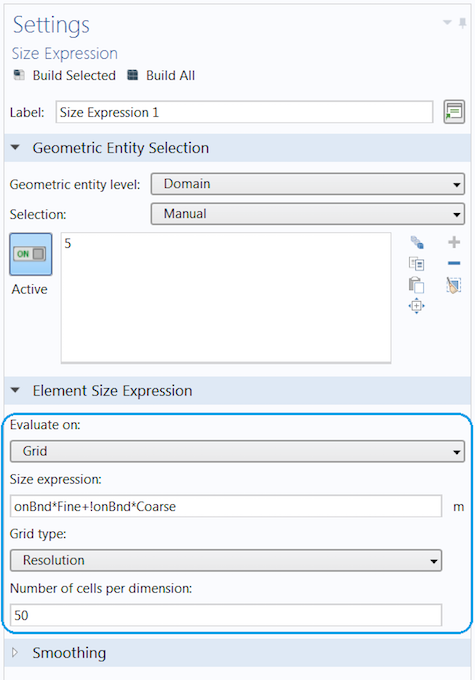
We use the default option, Evaluate on: Grid. This means that the expression is evaluated on a regular grid and interpolated between the grid points. This grid is not visible in the model but merely used to evaluate the size expression. When using this setting, it is important that all variables and functions used in the expression are defined under Global Definitions. We also increase the setting Number of cells per dimension to 50 (the default value is 25) to better resolve the region with a finer regular evaluation grid. Using any of the other options in the Evaluate on list gives the possibility to manually control the mesh on which the evaluation is done. The Size expression we use is defined as

onBnd*Fine+!onBnd*Coarse

where the two parameters, Fine and Coarse, are defined as 0.007 m and 0.07 m, respectively. When they are defined as parameters, they can be easily changed manually or varied in a parameter sweep by the Parametric Sweep study. There is a plot group called Mesh plot in the tutorial model that shows a cross section of the mesh used for the calculations. You can learn more in a previous blog post on visualizing mesh in greater detail.

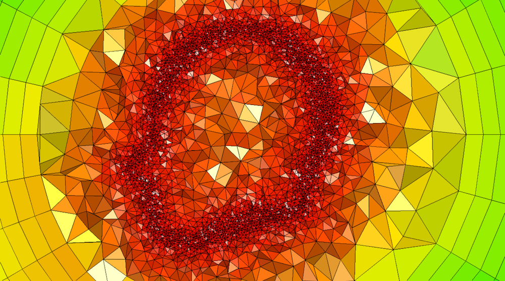
A mesh plot using a mesh Filter, plotting the mesh element size for x < 0. This image shows a much more refined mesh to make the plot clear. The tutorial model available for download uses a coarser mesh to save memory and time.

Setting Up the Materials and Physics

As mentioned above, we will only discuss the differences in setting up the materials and physics compared to the original tutorial. You can get details about the materials and physics used in the Specific Absorption Rate (SAR) in the Human Brain tutorial model. We keep Material 1 as the material for the antenna. A new material is added for the rest of the domains (the air and head). The material properties are defined using the interpolation functions k_int(x,y,z), epsr_int(x,y,z), mur_int(x,y,z), and sigma_int(x,y,z).

We select domain 5 (the air and head domain) to be active in the Bioheat Transfer physics interface. In the Bioheat subnode, two of the material properties for the blood are defined using the global variable avMat to make sure the value of the material properties is zero outside the head. For example, Specific heat, blood is defined as c_blood*avMat, where c_blood is a parameter. The Blood perfusion rate is set to the interpolation function omega_blood(x,y,z). We are now done with our modifications and are ready to compare the results after solving the model.

Comparing the Results and Discussing the Differences

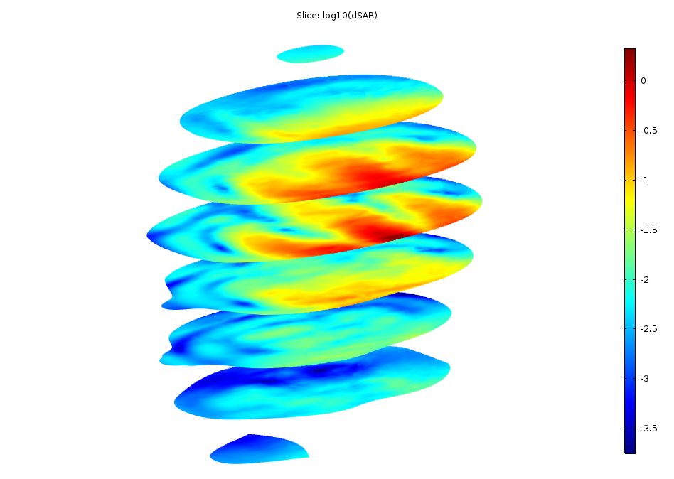
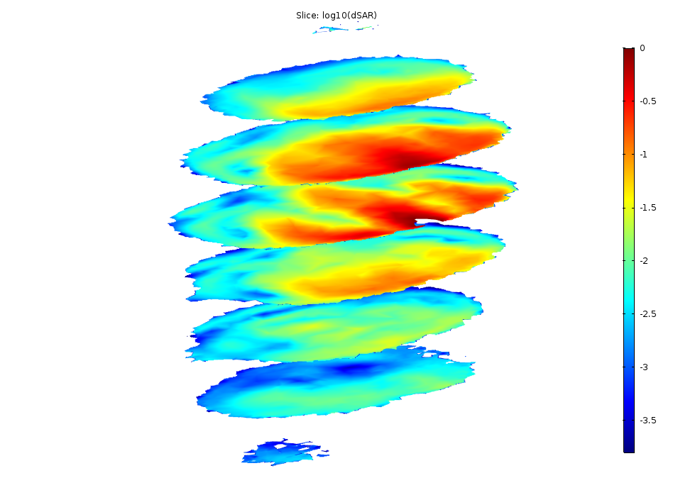
As seen in the images showing the SAR value, the radiation is absorbed in a similar manner in the two models. You can see the shape of the head in the slices, even though the edges of the slices are rather rough compared to the original model with the geometry object for the head. Manual color and data ranges are used for the plot in this tutorial, using interpolation functions to filter out the shape of the head.

Log-scale slice plot of the local SAR value. The left image shows the original tutorial and the right image shows the results from the model using interpolated materials.

We use a Volume maximum feature to calculate the maximum temperature rise in the head. This value is about 0.15 K in the original model and about 0.17 K in the model with the interpolated materials.

The two main components to get adequate results are:

1. Well-resolved material parameters
2. A fine-enough mesh, especially close to the surface of the head

It is possible to have material data that is much more resolved than the actual calculation mesh, but it will not help to make a finer calculation mesh if the material data isn’t resolved enough to match the calculation mesh. While a fine calculation mesh requires more memory and time to solve, better-resolved material data usually just takes more time to solve, as there is more data to interpolate from.

There is also another source of error: the fact that we are solving for bioheat transfer in the air with a small, nonzero thermal conductivity. However, this shouldn’t influence the results too much. The main sources of errors are the resolution of the material data and the calculation mesh.

Concluding Thoughts on Using Interpolated Material Data

In this blog post, we have shown how to set up a model with coordinate-dependent material properties defined in a text file, as well as how to adapt the mesh size to accurately resolve the border between two materials. We also discussed the sources of errors coming into play and how to improve the accuracy of the results. In a modeling scenario where we cannot generate the geometry of highly irregularly shaped objects, this approach can be a real lifesaver.

Next Steps

Try the tutorial model featured in this blog post by clicking the button below. From the Application Gallery, you can log into your COMSOL Access account and download the MPH-file.

• Check out the following resources for more information on modeling irregular shapes and using interpolation functions:
  • How to Build Geometries from Elevation Data to Model Irregular Shapes
  • How to Generate Random Surfaces in COMSOL Multiphysics®
  • Rock Fracture Flow