
In your finite element models, you may encounter the concept of numerical integration and Gauss points in several contexts. In this blog post, we discuss where and why numerical integration is used. Also, the possibilities you have to inspect and modify the numerical integration schemes in the COMSOL Multiphysics® software are highlighted. Finally, the use of Gauss point degrees of freedom is explained.
Table of Contents
- What Is Numerical Integration?
- Integration of Weak Contributions
- Modifying the Integration Order
- Built-In Reduced Integration
- Integration Coupling Operators
- Integration During Postprocessing
- Gauss-Point Shape Functions
- The gpeval Operator
What Is Numerical Integration?
When computing integrals of nontrivial functions over general domains, we must resort to numerical methods. Numerical integration is also called numerical quadrature. The idea is that the integral is replaced by a sum, where the integrand is sampled in a number of discrete points. This can be described as
where xi is the locations of the integration points and wi is the corresponding weight factors. The integration points are often called Gauss points, even though this nomenclature, strictly speaking, is correct only for integration points defined by the Gaussian quadrature method. In COMSOL Multiphysics, true Gaussian quadrature is used for integration in 1D, quadrilateral elements in 2D, and hexahedral elements in 3D. Other, similar schemes are used for other element geometries.
Gaussian Quadrature
In the Gaussian quadrature algorithm, the locations of the integration points and their weights are chosen so that a polynomial of as high of a degree as possible can be integrated exactly. Since a polynomial of degree N contains N+1 coefficients, and a Gauss point rule with M points contains 2M parameters (locations + weights), the highest order of the polynomial that can be integrated exactly is N = 2M – 1.
Gaussian quadrature is very efficient for integrating fields that can be well approximated by a polynomial of a certain degree. The integration points and weights for the first orders of Gaussian quadrature in 1D are shown in the table below. The integral is taken over the normalized interval [-1,1].
| Order (M) | Accuracy (N) | Location (xi) | Weight (wi) |
|---|---|---|---|
| 1 | 1 | 0 | 2 |
| 2 | 3 | ±0.577 | 1 |
| 3 | 5 | 0, ±0.775 | 0.889 (= 8/9), 0.556 (= 5/9) |
| 4 | 7 | ±0.340, ±0.861 | 0.652, 0.348 |
| 5 | 9 | 0, ±0.538, ±0.906 | 0.569, 0.479, 0.237 |
In COMSOL Multiphysics, integration orders are designated by the degree of the polynomial that can be exactly integrated. Only even numbers are used. For true Gauss point integration, the accuracy is, as shown above, always an odd power. The integration order designated by the software as “4” will actually have accuracy 5 on those element shapes where Gaussian quadrature is used.
Examples of Gaussian Quadrature
As an example of Gaussian quadrature, consider the function
Over the square -1 ≤ x ≤ 1, -1 ≤ y ≤ 1, the integral of this function is 1. As can be seen in the figure below, the function has a rather intricate distribution over the domain.
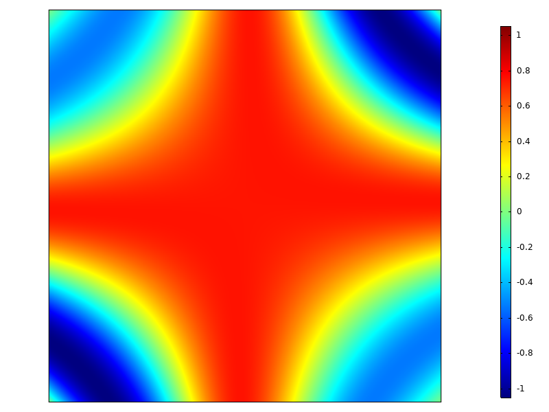
The function to be integrated.
In the table below, the results of different Gaussian quadrature orders are shown. As soon as the function can be reasonably approximated by a polynomial of a certain degree, the value of the integral converges fast.
| Integration Points | Accuracy | Integration Order | Value | Comments |
|---|---|---|---|---|
| 1 | 1 | 0 (or 1) | 2.9958 | Using only the value at the centroid clearly overestimates the integral |
| 2×2 | 3 | 2 (or 3) | 0 | In the 2×2 rule, the Gauss points are located at \pm \frac{1}{\sqrt{3}}, where the cosine function is 0 (bad luck!) |
| 3×3 | 5 | 4 (or 5) | 1.1519 | |
| 4×4 | 7 | 6 (or 7) | 0.9887 | |
| 5×5 | 9 | 8 (or 9) | 1.0005 | |
| 6×6 | 11 | 10 (or 11) | 1.0000 | |
| 7×7 | 13 | 12 (or 13) | 1.0000 | |
| 8×8 | 15 | 14 (or 15) | 1.0000 |
The optimal behavior of Gaussian quadrature for polynomials does, however, come with a downside: The method is not very good at integrating highly discontinuous functions. Suppose we want to integrate a function that equals f(x,y) = 1 when y < -2x – 1 and 0 elsewhere over the same square as above. Since the function has the value 1 over one quarter of the square, and the square has the area 4, we can immediately see that the exact integral should evaluate to 1. The results are shown in the table below.
| Integration Points | Value | Comments |
|---|---|---|
| 1 | 0 | Only one point at (0,0), where the function evaluates to 0 |
| 2×2 | 1 | One out of the four points evaluates to 1, and its weight is 1 |
| 3×3 | 0.8025 | Two points evaluate to 1, and their weights are \frac{25}{81}, \frac{40}{81} |
| 4×4 | 1.2269 | Five points evaluate to 1 |
| 5×5 | 1.0325 | |
| 6×6 | 1.0918 | |
| 7×7 | 0.9892 | |
| 8×8 | 0.9961 |

The case with 4×4 integration points. The orange surface is where the function has the value 1, and the green Gauss points are the ones contributing to the value of the integral.
As can be seen in the table, the effort to compute an accurate integral of this discontinuous function is significant. By pure chance, the 2×2 integration scheme gives the exact answer, but the convergence is far from monotonic.
Why is this important? In finite element analysis, you may encounter fields that exhibit sharp local gradients. Some examples are problems with phase transformations or at the onset of plasticity in solid mechanics. Integrals that are computed over elements containing these kinds of jumps may have significant discretization errors. Also, the convergence of the solution can be impaired. Small changes in the solution can significantly change computed residuals when individual Gauss points change their states.
In such cases, it may be better to select a lower polynomial order than the default for the shape functions used to discretize the field. The lower resolution can be compensated by using a denser mesh. The effect is that the inevitable jumps will be confined to smaller elements having fewer integration points.
Also, if you are computing integrals of discontinuous functions during postprocessing, the potentially slow convergence of numerical integration can be important to bear in mind.
Integration of Weak Contributions
Within each finite element, there are various expressions that need to be integrated in order to form, for example, stiffness matrices, mass matrices, load vectors, and residuals. Taking solid mechanics as an example, the standard weak (or variational) formulation corresponds to the principle of virtual work: The virtual work done by the internal stresses acting on a virtual strain variation equals the virtual work done by the external forces acting on the corresponding virtual variation of the displacements.
Here, the tilde (~) denotes the virtual variation. In an expression in COMSOL Multiphysics, this is represented by the test() operator. Volume forces, f, and boundary tractions, t, are included here, but there could also be other types of contributions. The left side will contribute to the stiffness matrix, while the right side will contribute to the load vector (assuming that the forces are independent of the displacements).
In order to inspect the formulations of the finite element implementations in COMSOL Multiphysics, you need to have Equation View enabled.
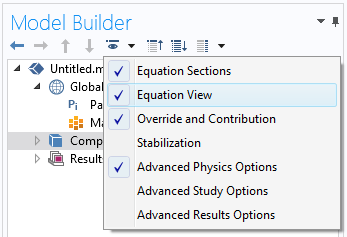
Switching on Equation View.
If we take a look in Equation View under a material model (say Linear Elastic Material) in the Solid Mechanics interface, there is a section named Weak Expressions. There, you can see the expressions used to form various matrices; for example, the stiffness matrix.
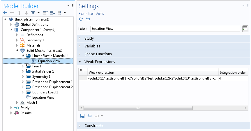
Inspecting the weak expression for the Linear Elastic Material in the Solid Mechanics interface in a stationary case.
In the figure above, you can see a text field for the integration order, which in this case has the value 4. The number describing the integration order in COMSOL Multiphysics is the highest order of the polynomial that can be integrated exactly. The default integration order is based on the order of the shape functions used to describe the field (in this case, the displacements). Here, the default shape function order — quadratic — is used, so stresses and strains will essentially have a linear variation over the element. The product of stress and strain variation is thus quadratic, indicating that order 4 could be more than necessary. Why this value is chosen will be discussed below.
As a second example, let’s examine a Boundary Load in Solid Mechanics.

The weak expression for Boundary Load.
Also here, the integration order is 4. Since the displacement shape functions are quadratic polynomials, it means that it should be possible to exactly integrate a load contribution for which the traction has no more than a quadratic variation, since the product of traction and variation of displacement is then of order 4.
Some Subtleties About the Weak Expressions
The discussion above is strictly true only if the elements have ideal shapes (e.g., no curved boundaries). If you delve into the theory, the integrals will actually also contain a local scale factor (Jacobian), coming from the transformation between the actual element geometry and the nominal element geometry. If, for example, an integral is performed over a 2D quadrilateral element, the numerical evaluation is done over the ideal square -1 ≤ ξ ≤ 1, -1 ≤ η ≤ 1,
The Jacobian will, in general, be a rational function (polynomials both in numerator and denominator), so it may not even be exactly integrable by this type of numerical quadrature. Because of this, it is wise to have some margin in the selected integration order. The Jacobian effect is, by the way, one reason why severely distorted elements perform worse than those with an ideal shape. This blog post on inspecting a mesh in COMSOL Multiphysics contains more information about mesh quality.
Even if an element shape function is called “quadratic”, it may (in some cases) contain higher-order terms. The shape function order indicated in the user interface shows the highest complete polynomial within the shape functions. The fact that there may be some higher-order terms present in the polynomials is another reason to use a more accurate integration rule than what would seem necessary at first glance.
Another reason that you may see a higher integration order than expected in Equation View for a certain contribution is that it may be necessary to ensure symmetry in a stiffness matrix.
Modifying the Integration Order
You can change the integration order for any weak expression from Equation View by editing the text field. There are two main reasons why you may want to do that.
The first is the more obvious one: You want to improve accuracy. Say that you have a load (in a general sense; this can be a force, heat flux, electric current, etc.) that has a variation that is fast when compared to the element size. Increasing the order of the numerical integration will then improve the accuracy of the total force or flux into the domain. The local solution close to where the boundary condition is applied, though, will still not be good, since it can never be better than what the shape functions of the element can represent.
There is, however, another interesting case: reduced integration, which means that the integration order, for some reason, is lower than what would formally be needed. One such reason is to speed up calculations. When solving a finite element problem, the majority of the CPU time is spent on two tasks: forming element matrices (assembly) and solving large systems of linear equations. The time spent on solving the equations increases faster than the model size, often approximately as the square of the number of elements. The time spent in assembly is directly proportional to the model size (actually, to the number of elements multiplied by the number of integration points per element). For a very large model, the equation solving will always dominate, but for medium-sized nonlinear models with heavy computations in each integration point, it may be worthwhile to consider the use of reduced integration.
Reduced integration is also a numerical device that is sometimes used to remove artificial stiffness that can appear in some element formulations in a phenomenon often called locking. One example where reduced integration is used for this purpose can be found in the Shell interface in 2D axisymmetry. In the virtual work equations, some terms are integrated with order 2 and others with order 4. If full integration was used everywhere, the element would actually be way too stiff when the shell thickness becomes small. By using reduced integration, some problematic terms in the strain energy are deliberately lost.

Virtual work contributions for the axisymmetric Shell interface.
Editor’s note: The following section was added on May 4, 2023 to include information about new functionality available as of version 6.0 of COMSOL Multiphysics.
Built-In Reduced Integration
Some of the Structural Mechanics interfaces include the option to select reduced integration directly from the settings of a certain material model.

The Quadrature Settings section in the Settings window for Linear Elastic Material.
There are several advantages to this approach when compared with editing the integration order in Equation View:
- The change can be made in one place and is automatically propagated to any possible subnodes.
- You don’t have to worry about what is the appropriate reduced integration scheme.
- For some element shape functions, the stiffness matrix will become singular if the integration order is lowered. This is mediated by the built-in Hourglass stabilization feature.
- Some material models, like plasticity, have local states stored at integration points. This is automatically synchronized with the integration rule.
Integration Coupling Operators
Under Definitions in the Model Builder, you can create integration operators. Such operators can be used to define global variables that are part of your problem formulation, but they can also be explicitly used in expressions during result evaluation.
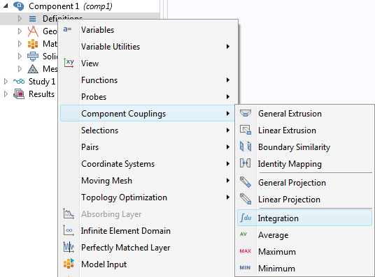
Adding an Integration operator.
When you add an integration operator, there are three main selections that you need to make:
- The domains, boundaries, or edges over which the integral should be taken.
- The integration order — This also gives you an option to trade accuracy for speed. Note that the actual integrand is not only the expression you supply, but that it is also multiplied by the Jacobian of the transformation from ideal to real element shape.
- The frame — This becomes important only when different frames exist, as with moving mesh, deformed geometry, and geometric nonlinearity in structural mechanics. Simply put: Should the integral be taken over a deformed or undeformed geometry?
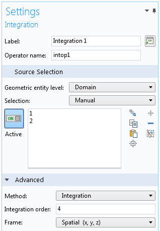
Settings for an Integration operator.
Integration During Postprocessing
When you want to compute an integral during postprocessing, you have two options: using an Integration operator (as described above) or adding an Integration node under Derived Values. To a large extent, the choice is arbitrary. However, in the Integration node, you cannot explicitly select the frame for the integration; it is inferred from the frame selection in the Data Set node.
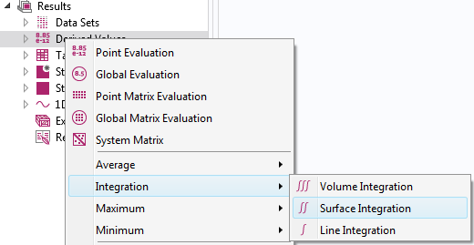
Adding a node for integration during result evaluation.
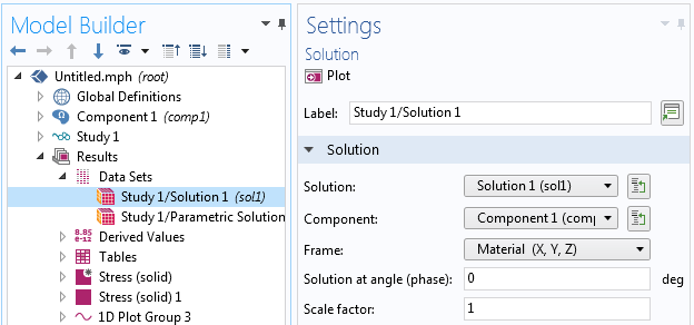
Settings for a dataset where the frame for result interpretation can be selected.
If the frame selection is important, you should probably rely on Integration operators to minimize the risk of making subtle errors. If you add an Integration operator after having solved the problem, you must run an Update Solution before the new operator is accessible.
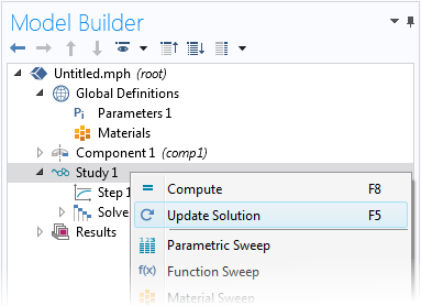
Updating a solution.
Remember to choose a high-enough integration order. In particular, be careful if the expressions to be integrated are strongly nonlinear or discontinuous. A common special case of discontinuous expressions is Boolean expressions. As an example, if after a heat transfer analysis, you want to compute the volume in which the temperature is above a certain value, you can use an integrand like T>1066[K]. This expression will evaluate to 1 where the condition is fulfilled and 0 elsewhere, so integrating it will give the volume where the condition is fulfilled. However, the border between the two values will, in general, cut through elements.
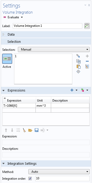
Integration of a Boolean expression with increased integration accuracy.
Gauss-Point Shape Functions
If you are making extensions to your multiphysics model, you sometimes need to add user-defined degrees of freedom (dependent variables). When doing that, you have to select the type of shape function used to represent them. One of the options is Gauss point data. All other options give different types of fields that have a continuous distribution over the element and may or may not be continuous between adjacent elements. The Gauss point data type of “shape function” is fundamentally different. It only stores a value at each Gauss point but has no connection to values elsewhere in the element.
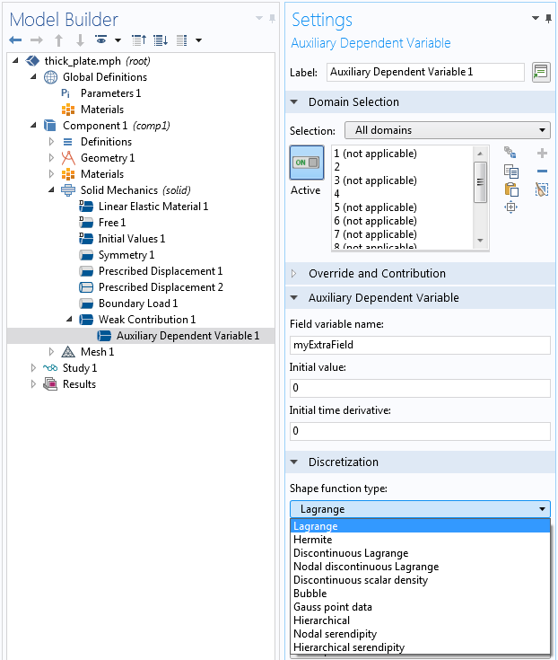
Selecting the type of shape function for a user-defined dependent variable.
The Gauss point data type is useful when you want to store a local state. This situation occurs in, for example, history-dependent nonlinear constitutive models requiring a “memory”. The constitutive model is mainly accessed when computing stiffness matrices and residuals, so the only locations in the element where it will actually be evaluated during the solution are at the integration points. Thus, it makes sense to store this type of data exactly there.
One example where Gauss-point data is used internally is for storing inelastic strains in material models, such as plasticity and creep in structural mechanics.
Once you have decided to store Gauss-point data, you need to select the Element order. In the case of Gauss-point data, this is the same as the integration order, discussed above. The cost (in terms of memory and CPU time) for storing Gauss-point data is proportional to the selected order in 1D, its square in 2D, and the third power in 3D.
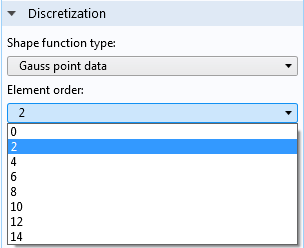
Selecting the integration point pattern.
If you are adding Gauss point variables to be used together with a built-in physics interface, you should usually select the same integration order as the one used for computing the relevant weak expressions. If there is a mismatch, values will have to be transferred between different locations in the element, with a loss in accuracy as well as performance.
The gpeval Operator
When you have variables stored in Gauss points, either built-in or defined by you, there are situations when you may need to interpolate them over the element. This is particularly important during postprocessing. As a default, the values of Gauss point variables are just picked from the closest Gauss point when evaluated at another location in the element. The gpeval() operator can be used to map the discrete Gauss-point data to a continuous field. In its simplest incarnation, the operator is referenced as gpeval(gporder, expression), for example, gpeval(4,solid.epe). For more details, please refer to the COMSOL Multiphysics User’s Guide.
As an illustration, consider the following example: the x-coordinate (ranging from 0 to 3) is stored as Gauss-point data in a small three-element model. This is done by adding an auxiliary dependent variable, as shown below.
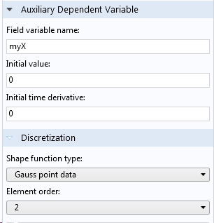

Storing the x-coordinate as Gauss-point data.
The weak contribution (myX-nojac(X))*test(myX) just states: “Set the variable myX equal to the current value of X.” The nojac() operator is added as a safeguard against getting a bidirectional coupling between myX and X. Using it is good practice when you just want to assign a value to a dependent variable.
If the Gauss point variable myX is then plotted as a surface plot (without averaging between elements), the result will be discontinuous. Within each element, the Gauss point variables are moved to the nearest corner and then interpolated over the element. If, instead, the expression gpeval(2,myX) is plotted, we retrieve the exact x-coordinate distribution.
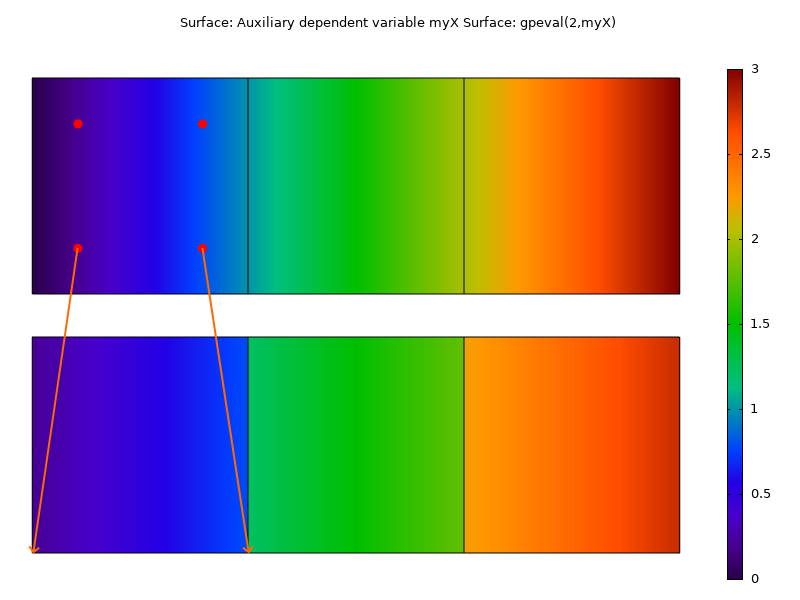
Plotting the Gauss point variable (bottom) and the extrapolated Gauss point variable (top). The arrows indicate how Gauss-point data by default is moved to the corners during result evaluation.
Next Step
Learn more about the functionality available in the COMSOL® software by clicking the button below:


Comments (4)
Yu Zhang
June 3, 2019Hi, Henrik:
Thank you for this useful blog. Could you please introduce a little bit more about the operator “nojac()”. You mentioned “The nojac() operator is added as a safeguard against getting a bidirectional coupling between myX and X”. What does this mean? Could you please introduce some situations when it is necessary to use this operator?
Thank you for your help.
Yu
Henrik Sönnerlind
June 4, 2019 COMSOL EmployeeHi Yu,
I will try to describe the nojac() operator somewhat, but in a bit sloppy way.
The name stands for ‘No Jacobian’. The operator makes sure that the expression inside the operator does not generate any contributions to the stiffness matrix. The expression will then only act as a right hand side in the system of equations. More formally: What is inside the operator is not differentiated with respect to the dependent variables.
Using a nojac() operator will in some cases have the same effect as using a segregated solver: The coupling in a segregated solver occurs only by passing residual between the dependent variables.
One way of thinking of it is to say that if you have two dependent variables ‘u’ and ‘v’ then a weak expression like (u-v)*test(u) can be interpreted as ‘u=v’, while (u-nojac(v))*test(u) can be interpreted as ‘u <- v'. This is how I use it in the blog post. If you are just using a dependent variable for storing a value, it is good practice to make sure that the assignment operation does not affect the value to be stored.
There are several other possible uses for the nojac() operator. One is to just drop some terms in the stiffness matrix that are expensive to compute, but not important for the convergence. Similarly, you could use it to drop terms that give you an unsymmetric stiffness matrix.
It should be noted that using nojac() will have effects on the solver. The use of nojac() will cause the problem to be treated as nonlinear. If you know that this is not the case, you will have to use a segregated solver with a smart setup in order to avoid performing extra solutions.
Regards,
Henrik
Casper Kerkhove
October 4, 2024Hey Henrik,
Thanks for the post! There is one thing I cannot figure out though. I have defined some control-variable field w.r.t. which I am performing a sensitivity analysis. Of the field itself, however, I would really like to be able to obtain the list of its Gauss-point weights. As a work-around, I could define a “Volume” objective that simply integrates 1 over the domain of this field, and then calculate the sensitivity with respect to this field, but that seems impractical and I would like to avoid that if there is any other way to obtain these weights directly. Another reason why I prefer not to calculate this volume sensitivity is that Comsol seems to require a separate study, also with some physics to be present in the study step. But any physics and its solution are technically wasting computational effort, unless I define some custom weak-form whose system matrix is equivalent to the volume gradient. But now I am just stacking work-arounds ): Sorry for the long question, and thanks in advance!
Kristian Ejlebjærg Jensen
October 8, 2024 COMSOL EmployeeHi
I have answered your question in the forum: https://www.comsol.com/forum/thread/344961/multiple-sensitivity-analysis-steps-per-study
Best regards,
Kristian