
The nonlinear magnetic saturation curves in the AC/DC Module’s Nonlinear Magnetic Materials Database can now be used in frequency-domain simulations using COMSOL Multiphysics version 5.2. You can now convert the associated B-H or H-B curve, which was previously supported only for stationary and time-dependent studies, into an effective B-H or H-B curve using the newly added Effective Nonlinear Magnetic Curves Calculator app. In this blog post, we will discuss how this app is used in frequency-domain simulations.
Nonlinear Magnetic Materials in the Frequency Domain
A common modeling assumption is to specify the linear magnetic permeability in the constitutive relation. It is often a good practice to assume that the material responds linearly with respect to the applied field in the initial modeling stage. In COMSOL Multiphysics, this can be done by simply applying a constant value for magnetic permeability within the constitutive equations in the magnetic interfaces.
However, many ferromagnetic materials exhibit nonlinear behavior, as the magnetization depends nonlinearly on the magnetic fields, even for a small change. These materials also exhibit hysteresis, a history dependence of the applied magnetic field on magnetization. Modeling hysteresis behavior is computationally demanding and difficult. The nonlinear magnetic materials available in COMSOL Multiphysics do not include the full hysteresis loop, but instead, the average B-H curve that incorporates magnetic saturation effects in the first quadrant, as discussed in this blog post.
These magnetization curves are also called dc or normal magnetization curves, which are obtained by plotting the locus of the maximum values of B and H at the tips of the hysteresis loops. These magnetic saturation curves can be used directly in the stationary and time-dependent studies, but not for the frequency domain. To solve in the frequency domain, you would need a “cycled averaged” B-H/H-B curve that approximates a nonlinear material at the fundamental frequency.
The Effective Nonlinear Magnetic Curves Calculator app can be used to generate the effective B-H/H-B curves for frequency-domain (time-harmonic) simulations. These effective B-H/H-B curves can be directly used in the magnetic interfaces in the AC/DC Module in COMSOL Multiphysics version 5.2, which has built-in support for these materials.
Note: The full hysteresis loop can be implemented in COMSOL Multiphysics by adding extra partial differential equations (PDEs) to describe the material models; for example, the Jiles-Atherton model in the time domain. A 3D time-domain model demonstrating the Jiles-Atherton vector hysteresis model is available in the Application Gallery. In addition, the AC/DC magnetic interfaces in COMSOL Multiphysics version 5.2 support material models defined in external C code. This allows the app creator to have the app user define subroutines to describe material models; for example, by implementing the full hysteresis loop and using those material models in a magnetic simulation in full 3D geometry. The example demonstrating the C code material model is available here.
Editor’s note: We published a blog post about the implementation of the external material models for magnetic simulation on 3/10/16. Read “Accessing External Material Models for Magnetic Simulations” to learn more.
Exploring the Effective Nonlinear Magnetic Curves Calculator App
Magnetic interfaces in the AC/DC Module of COMSOL Multiphysics version 5.2 now support the effective H-B/B-H curve material model, which can be used to approximate the behavior of a nonlinear magnetic material in a frequency-domain simulation without the additional computational cost of a full transient simulation. To be able to use this new effective H-B/B-H curve material model, we require the effective Heff(B) or Beff(H) relations, defined as an interpolation function.
This utility application can be used to compute the interpolation data starting from the material’s H(B) or B(H) relations. The interpolation data for the H(B) or B(H) relations can be imported from a text file or entered in a table. The application can then compute the interpolation data for the Heff(B) or Beff(H) relations using two different energy methods: Simple Energy and Average Energy. When using the AC/DC Module, the output result plots of effective H-B/B-H curves can be exported either as a text file or as a Material Library file that can be imported into COMSOL Multiphysics for the frequency-domain simulation of magnetic materials.
User Interface
The user interface consists of four different sections: Ribbon, Material Information (Input & Results), Curve Plots, and Curve Analysis, as shown in the image below. The material data for the magnetic flux density (B) and magnetization field (H) can be directly typed in the table or imported from a text file using the Import Curve Data button on the menu.
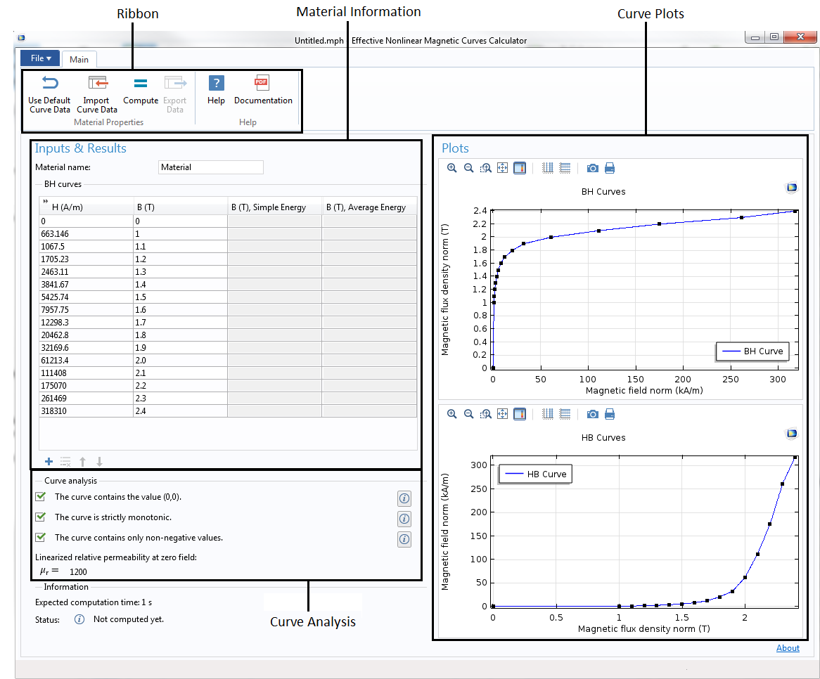
The customized user interface for the Effective Nonlinear Magnetic Curves Calculator app.
The Ribbon section contains six buttons for different operations. Click on the Use Default Curve Data button to use the default input B-H curve that is already loaded in the application. If you wish to bring in your own curve, click on the Import Curve Data button to open the Import Curve dialog box (as shown below) and import a text file containing the interpolation data for the B-H or H-B curve. In the Import Curve dialog box, specify the file to import by clicking on the Browse button.
The text file must contain pairs of values separated by whitespace characters or commas, with one pair for each line. Choose either B-H Curve or H-B Curve from the Import curve as combo box. For a B-H curve, the first column represents H values and the second column represents B values and vice versa for an H-B curve. The default data table will be replaced with the imported data, which, if needed, can be edited in the table. Rows can be added or removed using the buttons below the table.
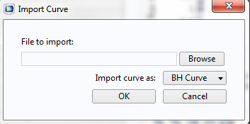
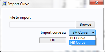
Dialog box for the Import Curve Data button in the Ribbon section.
In the Curve Analysis section, curve data is automatically analyzed each time the data is modified or imported from the file. Curve analysis includes three conditions that the imported data must satisfy: the curve must contain the value (0,0); the curve must be strictly monotonic; and the curve must be nonnegative. If any of these conditions are not fulfilled, modify the values in the table to correct the problem. The linearized permeability at zero field (the slope of the curve at H = 0) is also computed and displayed.
Once the data is modified or imported, click on the Compute button in the ribbon to compute the effective curves using the Simple Energy and Average Energy methods. The computed values for the effective B field for both the Simple Energy and Average Energy methods are displayed in the last two columns of the table. The plots for the original B-H and H-B curves as well as the Heff(B) and Beff(H) curves for both methods are displayed in the graphics window, as shown below.
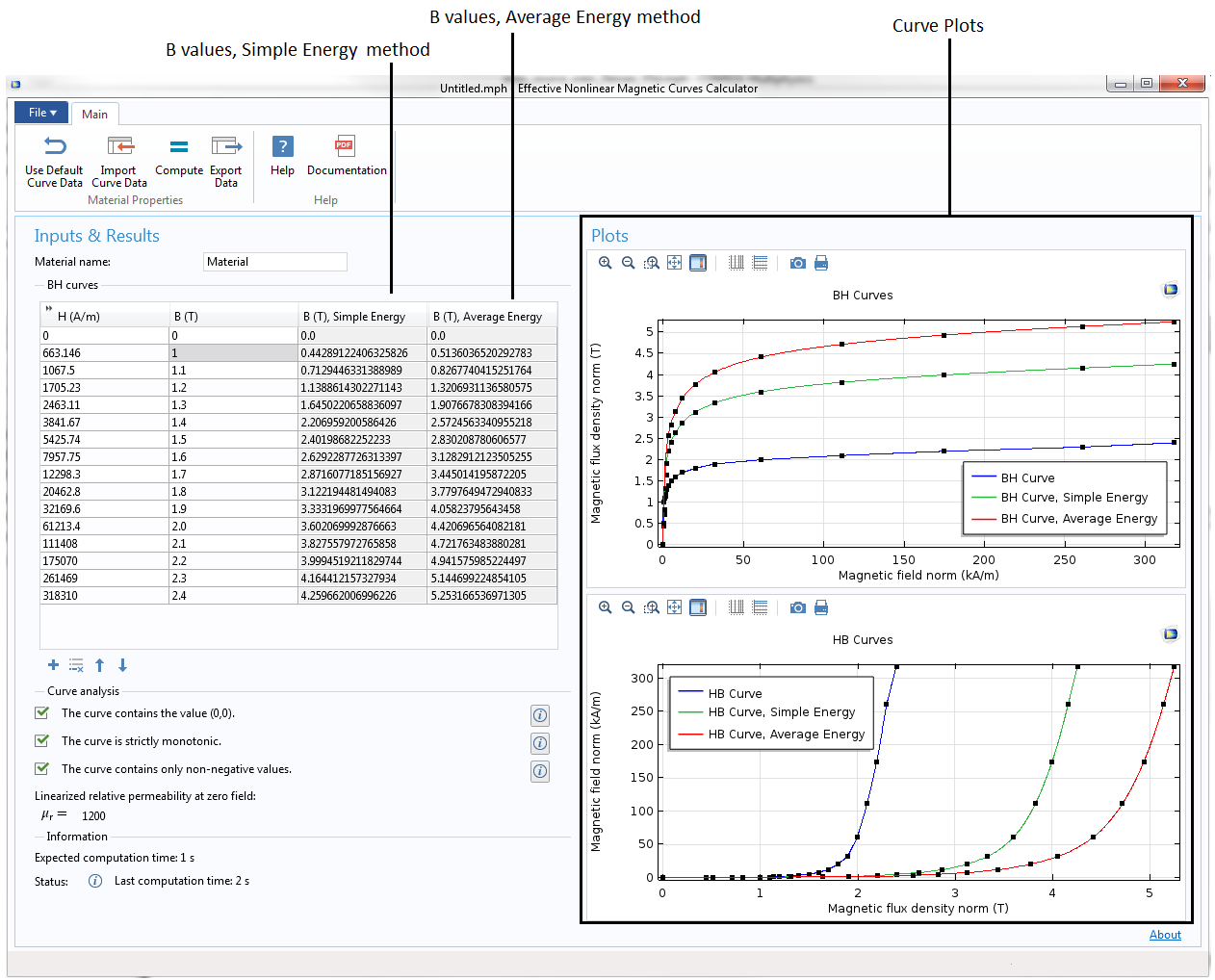
The app’s user interface, displaying the computed data and plots for magnetic curves.
The computed interpolation data for the effective H-B/B-H curves can be exported for further use in other COMSOL Multiphysics applications. Click on the Export Data button in the ribbon to open the Export Material Data dialog box. You can export the data as a text file or to the Material Library by choosing the respective option in the Export as combo box.
In the Text File export option, you could choose any one of the averaging methods and curve types. This exported text file contains a pair of values in each line. This text file can be imported, for example, in an Interpolation Function node in a COMSOL Multiphysics application and used for defining the effective H-B/B-H curve for frequency-domain magnetic simulations.
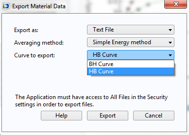
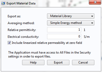
The Export Material Data dialog box, illustrating the Text File (left) and Material Library (right) data export options.
You could also export the curve data as a COMSOL Multiphysics Material Library file by using the Material Library export option in the Export as combo box (see the image above, on the right). The material in this exported Material Library file contains the H-B curve, B-H curve, effective H-B curve, and effective B-H curve based on the selected averaging method (Simple Energy or Average Energy). You could also include the linearized relative permeability by selecting the Include linearized relative permeability at zero field check box. The exported Material Library file can be added into the Material Library, as shown in the picture below.
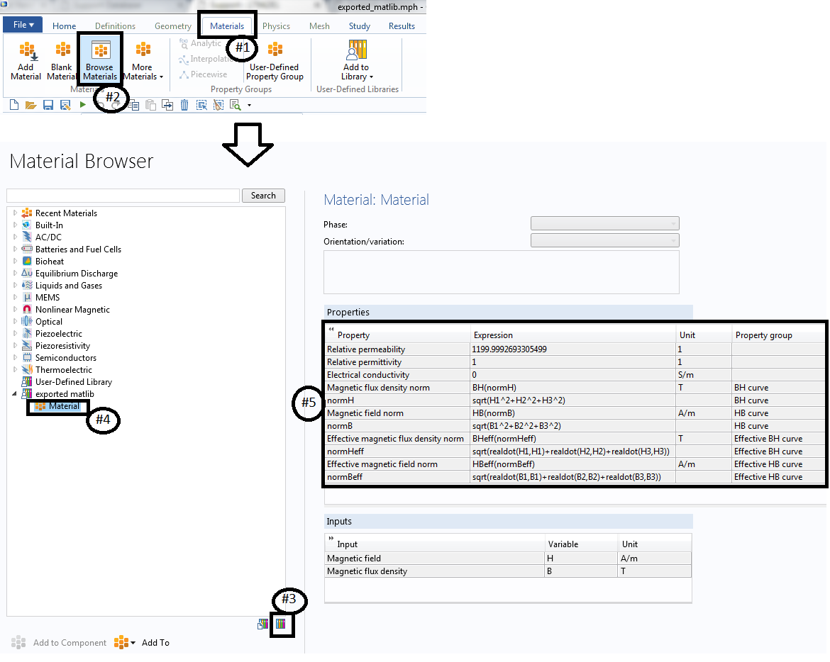
The Material Browser window, showing the steps for adding the exported Material Library file into the Material Library.
Note: You can now use any of the materials that are available under the Nonlinear Magnetic folder in the COMSOL Multiphysics Material Library for a frequency-domain simulation by first converting the available H-B/B-H curves into effective H-B/B-H curves using this utility app. Simply add the material in the COMSOL Multiphysics model, export the B-H curve or H-B curve data as a text file, import the text file into the Effective Nonlinear Magnetic Curve Calculator app, evaluate and export the effective H-B/B-H curves, and finally import the effective H-B/B-H curves into the same COMSOL Multiphysics model for frequency-domain simulations. The Soft Iron (with losses) and Soft Iron (without losses) materials under the AC/DC folder already contain the effective H-B/B-H curves, which can be used directly in frequency-domain simulations.
The Embedded Model
The embedded model in this app computes the effective nonlinear magnetic curves for materials using the Simple Energy and Average Energy methods. The integration expressions for calculating effective magnetic flux density strengths are given below. The integration method available in this app is selected based on the paper by Gerhard Paoli, Oszkár Biró, and Gerhard Buchgraber.
where H is the amplitude of the time-harmonic magnetic field, B(H) is the material’s nonlinear B-H relation, H(t) is the time-dependent oscillating magnetic field, and T is the arbitrary period of oscillation.
For more information about the model, refer to the PDF document by clicking on the Documentation button in the ribbon of the app.
Using the Effective H-B/B-H Curve
To illustrate this new effective H-B/B-H curve material model in COMSOL Multiphysics version 5.2, let’s take a look at the square-shaped, closed, magnetic core excited by the multiturn coil on one arm, as shown in the image below, on the left. The magnetic core is modeled in the Magnetic Fields physics interface using Ampère’s Law, with three different material types: nonlinear H-B curve, nonlinear effective H-B curve, and linear material.
The first nonlinear H-B curve model is solved in the time domain, whereas the other two material models are solved in the frequency domain at 1 kHz. The magnetic flux density at one of the corners inside of the magnetic core is measured and compared for all three different material models; see the image below, on the right. As expected, the effective H-B/B-H curve model behaves much closer to that of the nonlinear H-B/B-H curve model in the time domain. However, the time-domain model still exhibits the higher harmonics, unlike the other two models. The linear material model is quite different compared to the other two models. Therefore, for many applications where the higher harmonics are not important, the effective H-B/B-H curves can be appropriate, as they are less computationally expensive. You can download this example here.
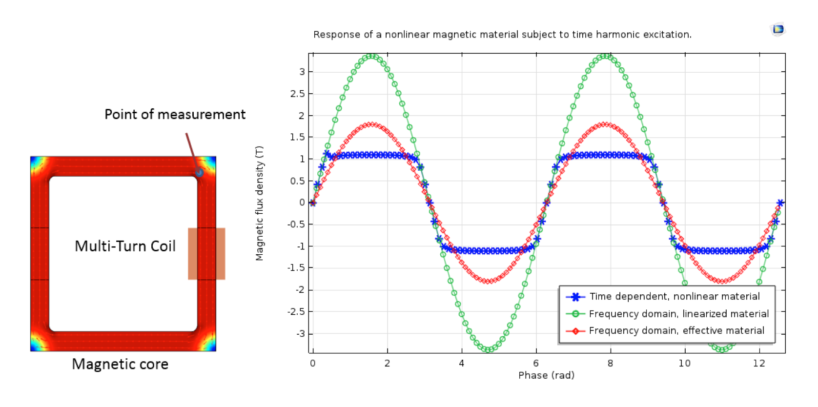
The magnetic flux density norm surface plot on the magnetic core (left). A comparison of the magnetic flux density norm at a point inside of the magnetic core for three material models (right).
Concluding Remarks
In this blog post, we have discussed the various material models available for modeling nonlinear magnetic materials. We also detailed the Effective Nonlinear Magnetic Curves Calculator application and explained how to utilize this app to generate the cycled-average effective H-B/B-H curves for the frequency-domain simulation of magnetic devices. Finally, we demonstrated an example using three types of material models (B-H/H-B curves, effective H-B/B-H curves, and linearized material) and compared the results.
If you are interested in modeling nonlinear magnetic materials for time-harmonic or time-dependent studies, please contact us.
Reference
- Gerhard Paoli, Oszkár Biró, and Gerhard Buchgraber. “Complex representation in nonlinear time harmonic eddy current problems,” Magnetics, IEEE Transactions, vol. 34.5, pp. 2625-2628, 1998.
Try It Yourself
- Try the new Effective Nonlinear Magnetic Curves Calculator app
- Download the Comparison of Effective H-B/B-H Curve with Linear and Nonlinear Material Models example
- Read a related blog post: “Accessing External Material Models for Magnetic Simulations“


Comments (1)
Dag Willen
April 19, 2016Thanks for this excellent example. The links to the relevant .mph example helped to understand the final details to make Comsol compute with the effective BH tables.