

The exotic electromagnetic properties of metamaterials are of significant interest to researchers. Metamaterials enable nanoscale manipulation of light in unprecedented ways with extreme control over the field properties. In this blog post, we discuss the setup of a simulation to excite a hyperbolic wave in a metal–dielectric layered metamaterial and calculate the effective permittivity of the structure.
Introduction to Metamaterials
Metamaterials are artificially engineered structures composed of subwavelength building blocks. These structures exhibit anisotropic dispersion, and their electrical properties, such as permittivity, permeability and conductivity, can be controlled by changing the shape, geometry, size, orientation, and material properties of the composing unit cells. With adequately chosen control parameters, metamaterials can be designed to behave as a metal (negative real permittivity) or dielectric (positive real permittivity). The metallic or plasmonic metamaterials exhibit two different topologies: hyperbolic and elliptic. In hyperbolic typologies, the permittivities in the orthogonal axes are of opposite signs; in elliptic topologies, the permittivities are negative in all directions.
This type of plasmonic metamaterials can be constructed using periodically organized metal–dielectric layers and metallic nanorods embedded in a dielectric, with subwavelength periodicity and dimension. The hyperbolic waves propagating within the metamaterial structure are extremely confined, and their wavelengths can be 100 times smaller than the free-space wavelength. Such distinctive electromagnetic features set hyperbolic metamaterials apart from the conventional isotropic materials in potential applications, such as enhanced superlensing effect, subdiffraction imaging, sensing, negative refraction, energy harvesting, and quantum and thermal engineering.
In the following section, we discuss the semiclassical electromagnetic approach to calculate the permittivity tensor components of a metal–dielectric layered metamaterial.
Calculating Metamaterial Permittivity: Simulation vs. Effective Medium Theory
Let us consider that a linearly (vertically) polarized electric point dipole source is located in air near a hyperbolic metamaterial composed of periodically oriented subwavelength metal–dielectric layers. The evanescent fields radiated by the dipole couple to the structure and excite two types of waves: surface plasmon polariton, which propagates along the metal–air interface, and hyperbolic wave, which propagates within the metamaterial.

Schematic of an electric point dipole located in air near a metamaterial structure. The structure is composed of periodically organized metal and dielectric layers with subwavelength thickness and periodicity.
The anisotropic relative permittivity tensor \varepsilon of the metamaterial can be calculated by solving the constitutive relation. It can be written in terms of the electric displacement field \textbf{D} and the electric field \textbf{E} as
1
Assuming that the metamaterial is nonmagnetic, the radial and vertical components of \varepsilon can be expressed as
2
3
Equations 2 and 3 permit to calculate the metamaterial permittivity tensor when \textbf{D} and \textbf{E} are known. To evaluate these values in the COMSOL Multiphysics® software, we use up and down operators to calculate the average electric displacement field and electric field components. Then, the average operator is used to perform integration of the constitutive relation \textbf{D}=\varepsilon\textbf{E} to calculate the effective permittivity. It is important to highlight that these operators are performed on the metal–dielectric interior boundaries within the metamaterial to evaluate fields with discontinuity on each side of the boundaries.
An alternative approach to calculate the metamaterial permittivity is the effective medium theory. Within the subwavelength regime, the diagonal components can be calculated using the effective medium theory as1
4
5
with F_m = t_m/(t_m+t_d) being the filling ratio of metal. Here, t_m and t_d are thicknesses of metal and dielectric layers, respectively; and \varepsilon_m and \varepsilon_d are relative permittivities of metal and dielectric, respectively.
Equations 4 and 5 show that the anisotropic dispersion of the metamaterial depends on the thickness of the metal–dielectric layers and the filling ratio. The values of \varepsilon_{rr} and \varepsilon_{zz} can be positive or negative, depending on the layer thickness, and material properties.
For further demonstration, assume a metamaterial composed of silver (metal) and silicon dioxide (dielectric). The real parts of the diagonal components of the relative permittivity tensor are plotted below versus the metal filling ratio, F_m, indicating the dielectric, hyperbolic, and elliptic regimes. Here, \varepsilon_{zz} displays a resonance behavior as it depends on the electromagnetic coupling between the adjacent metal layers, whereas \varepsilon_{rr} shows a smooth variation. Within the hyperbolic regime, the permittivity tensor components are of opposite signs. In the case of larger F_m, the value of \varepsilon_{zz} is dominated by the increased volume of metal, and it is negative, which generates the elliptic topology. When F_m is very small, the influence of metal is negligible on the metamaterial properties and it behaves as an anisotropic dielectric medium.

Real part of diagonal components of the effective relative permittivity of the metamaterial as a function of metal filling ratio. The metamaterial is composed periodically organized silver and silicon dioxide layers with subwavelength thickness and periodicity.
The following section details the simulation set up to excite hyperbolic waves in the metamaterial.
Simulating the Hyperbolic Wave Excitation
This section discusses the capabilities of the COMSOL Multiphysics® software to simulate hyperbolic waves propagating in a metamaterial using the field radiated by an electric point dipole located nearby. The metamaterial is made of thin layers of periodically organized silver and silicon dioxide, with material properties taken from the software’s built-in material library. The Electromagnetic Wave, Frequency Domain interface with 2D axisymmetric geometry, part of the Wave Optics Module add-on product, is used for this model. The electric point dipole is defined using a Weak Contribution node, as indicated in the following screenshot, and perfectly matched layers are employed to absorb the waves and minimize unwanted reflections. One wavelength domain study step is used to solve for the domain fields. An additional wavelength domain study step is performed to calculate the effective permittivity tensor of the metamaterial versus wavelength. The permittivity tensor components computed from the effective medium theory using Equations 4 and 5, and from the constitutive relation using Equations 2 and 3, are calculated versus free space wavelength.

Weak contribution is used at the source point to define the electric field radiated by a linearly (vertically) polarized electric point dipole. Wavelength domain study steps are used to solve the domain fields and the metamaterial dispersion.
Results
After running Study 1 of the simulation, the hyperbolic waves excited in the metamaterial can be visualized. The animation below shows the instantaneous electric field at 2.6 eV photon energy. As detailed above, the dipole excites hyperbolic modes propagating within the metamaterial and surface plasmon polariton at the metamaterial–air interface propagating away from the source point in the radial direction.
Simulated instantaneous electric field of the hyperbolic wave excited in the metamaterial and surface plasmon polariton propagating at the metamaterial–air interface.
The effective relative permittivity of the metamaterial can be calculated after running Study 2 of the simulation. Results are calculated using the effective medium theory and by computing the constitutive relation from Equations 2 and 3, and they are in excellent agreement as shown below.

Diagonal components of the metamaterial effective permittivity calculated using the effective medium theory (solid lines) and from simulation (markers).
To further visualize how the field profile changes as a function of photon energy, the animation below shows the electric field norm of the hyperbolic wave when the photon energy changes from 2.6 eV to 1.4 eV. This illustrates how the branches of the hyperbolic wave evolve with photon energy.
Variation of hyperbolic waves inside the metamaterial as a function of photon energy from 2.6 eV to 1.6 eV.
The information in this blog post can be used to model different types of plasmonic materials in COMSOL Multiphysics® and explore the associated light–matter interaction.
Try It Yourself
Want to try modeling a hyperbolic wave in a metamaterial? Download the model discussed in this blog post via the link below.
Reference
- T. Li and J.B. Khurgin, “Hyperbolic metamaterials: beyond the effective medium theory”, Optica 3, pp.1388–1396, 2016
Further Reading
- For more information about metamaterials, read the following blog posts:


Comments (0)