

The katana is a legendary sword used by the samurai several hundred centuries ago. It is perhaps most recognizable for its curved shape and its remarkably sharp single edge. In this blog post, we will go over how to build a simple model of a katana using the COMSOL Multiphysics® software and simulate a differential hardening process to explore some of its features.
Table of Contents
- The Famous Katana
- The Metal Processing Module
- Differential Hardening
- The Multiphysics of Heat Treatment
- The Material of the Katana
- Geometry of the Katana
- Phase Transformation Modeling:
- Mechanical and Thermal Material Properties
- Heat Transfer Modeling:
- Stress and Strain Modeling
- Results
- Applying What We Learned
The Famous Katana
Few weapons are as famous as the katana — the sidearm of the Japanese samurai warriors. Notorious for its sharpness and unsheathed only as a last resort, the sword, and its almost sacred connection with its owner, has inspired several modern-day films, TV series, and books. In the films Kill Bill I (2003) and Kill Bill II (2004), Uma Thurman’s character ‘the Bride’ wields a katana in modern-day Tokyo, and in James Clavell’s classic novel Shogun (1975), captain James Blackthorne is blown ashore on the coast of Japan and taken captive by samurai.
A photograph of a samurai, taken by photographer Felice Beato, c. 1860. This image is in the public domain in the United States because its copyright in Japan expired by 1970 and was not restored by the Uruguay Round Agreements Act . Source: Britannica.
The katana, of course, gained most of its notoriety while in the hands of its user. But how did the Japanese swordsmiths make these weapons for the samurai? How did they achieve the delicate balance between hard and soft parts of the blade, to make the katana razor sharp, yet ductile enough to endure repeated strikes? Why is the blade of a katana curved, and not straight? In this blog post, we will cover how to model the differential hardening process of a katana and examine the effects to see if we can gain some insight into the making of this historically famous weapon.
The Metal Processing Module
The Metal Processing Module, an add-on product to COMSOL Multiphysics®, can be used to model phase transformations in ferrous alloys like steels, and in titanium alloys such as Ti–6Al–4V. Applications include steel quenching and additive manufacturing. Steel quenching enables you, for example, to model hardening of automotive transmission components, while additive manufacturing can involve the repeated cooling–heating cycles that occur during printing. The phase transformation modeling capability is supplemented with couplings to the fields of solid mechanics and heat transfer, enabling effects like plasticity and latent heat of phase transformation.
Differential Hardening
In many situations, it is desirable to harden only parts of a component. One example is induction hardening. A strong alternating magnetic field is applied using electric coils, whereby electric currents are induced at the surface of the component. The component is then quenched, and the surface region undergoes martensitic transformation. This differential hardening process is often used for transmission components like axles and gears for the purpose of increasing the wear resistance and fatigue resistance.
Flame hardening is another process that can be used to obtain a hard surface of a component. Instead of an alternating magnetic field, the surface is locally heated by gas flames that are exerted on the surface, followed by quenching.
Of course, induction hardening and flame hardening are relatively novel heat treatment processes that were not available to Japanese swordsmiths many centuries ago. In traditional Japanese katana making, another type of differential hardening was used. For a sword of this type, it is beneficial if the sharp edge of the blade is hard — ideally purely martensitic. At the same time, the ridge of the blade is preferably ductile, for example, pearlitic; otherwise the sword may break on impact. The traditional way to differentially harden a katana is to apply insulating clay to the blade, so as to affect the heat transfer from the hot steel to the surrounding water as it is being immersed. Different regions of the blade are cladded with clay of different thicknesses. Near the edge, a thinner layer of clay is used compared to the remaining parts of the blade, where a thicker layer is applied.
The Multiphysics of Heat Treatment
Simulating the heat treatment of a steel component requires you to identify the physics phenomena that are relevant to include in the model.
Fundamentally, the process is driven by heat transfer due to the heat exchange with the exterior. The change in temperature inside the component, the katana in this instance, induces metallurgical phase transformations (decomposition of austenite into ferrite, pearlite, etc.). During phase transformations, latent heat is produced, which affects temperatures. The volume changes associated with thermal expansion and density differences between phases result in distortions of the component, as well as mechanical stresses and plastic strains. In turn, it is known that phase transformations that occur in the presence of mechanical stresses cause inelastic strains in the material, so-called transformation induced plasticity (TRIP). The quenching process is truly multiphysics in nature, and to complicate matters further, the individual metallurgical phases have different material properties producing an averaged, phase-composition-dependent, compound material behavior.
In the present model of the heat treatment of a katana, the following simplifications are made:
- Latent heat during phase transformations is neglected
- TRIP strains are neglected
The heat treatment of the katana is visualized in the figure below.
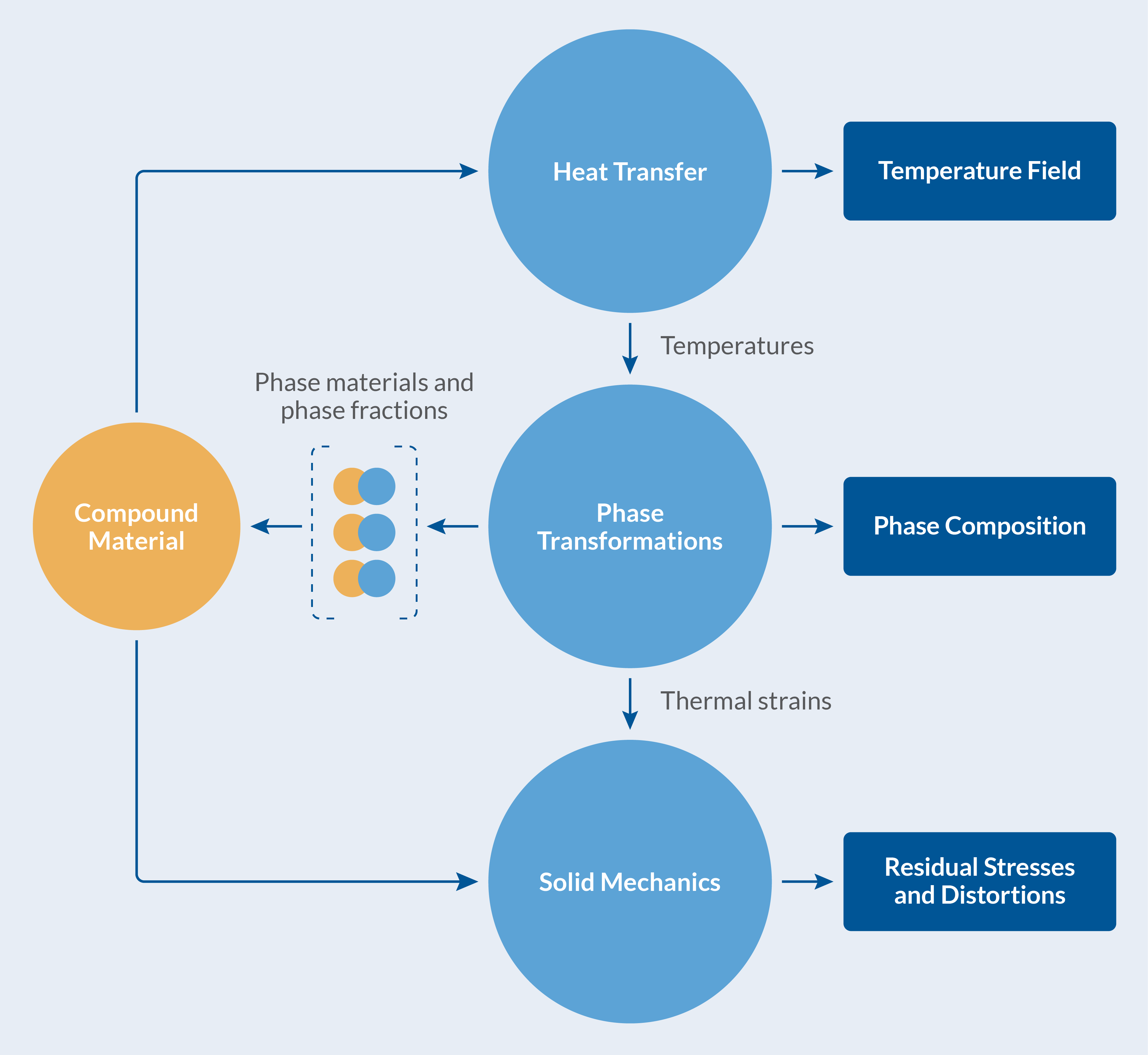 The multiphysics of the heat treatment of a katana.
The Material of the Katana
The traditional way of making a katana involves using different steel types for different sections of the blade. Typically, the edge is different from the core of the blade, and the most notable difference is in the varying carbon content. The amount of carbon, as well as other alloying elements, strongly affects both the thermal and mechanical properties of the steel, as well as the phase transformation characteristics. Here, a simplification into a single steel type has been made. Its alloying content is given in the table below:
| Element | wt% |
|---|---|
| C | 0.63 |
| Mn | 0.9 |
| P | 0.04 |
In reality, a steel would contain additional alloying elements, but for the sake of simplicity, we only consider manganese (Mn) and phosphorus (P), in addition to carbon (C).
Geometry of the Katana
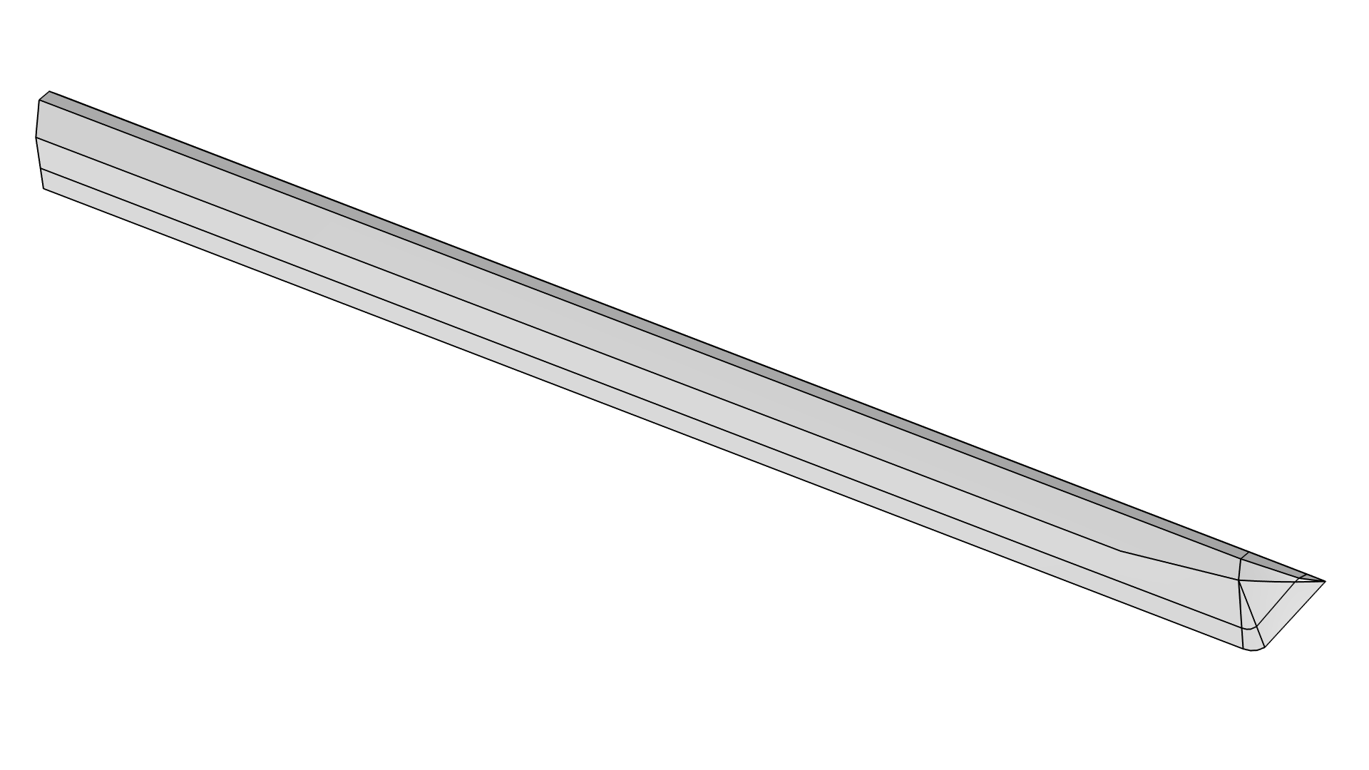
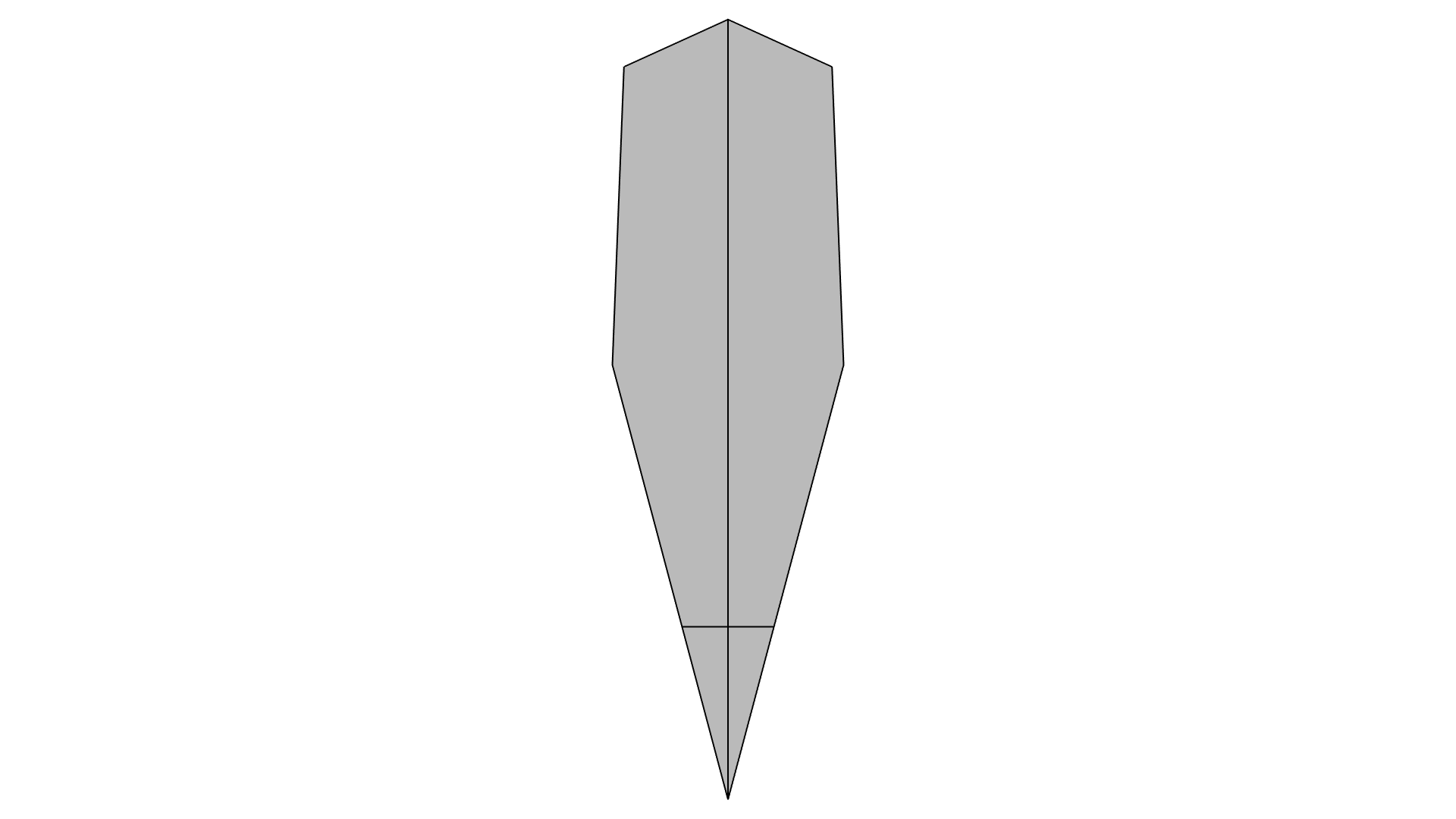
The geometry of the katana: The blade is 50 cm in length (left) and a cross section of the blade is 2.8 cm in height (right).
Phase Transformation Modeling
The various possible phase transformations have to be characterized. At room temperature, the steel is considered to have a base composition of 50% ferrite and 50% pearlite. The katana is first heated until this base composition has been fully transformed into austenite. The katana is then quenched in water to obtain a final phase composition. This composition will vary spatially, and will in general be some combination of ferrite, pearlite, bainite, martensite, and possibly retained austenite. See the figure below. The spatial variation is affected by the thermal history at each material point during cooling.
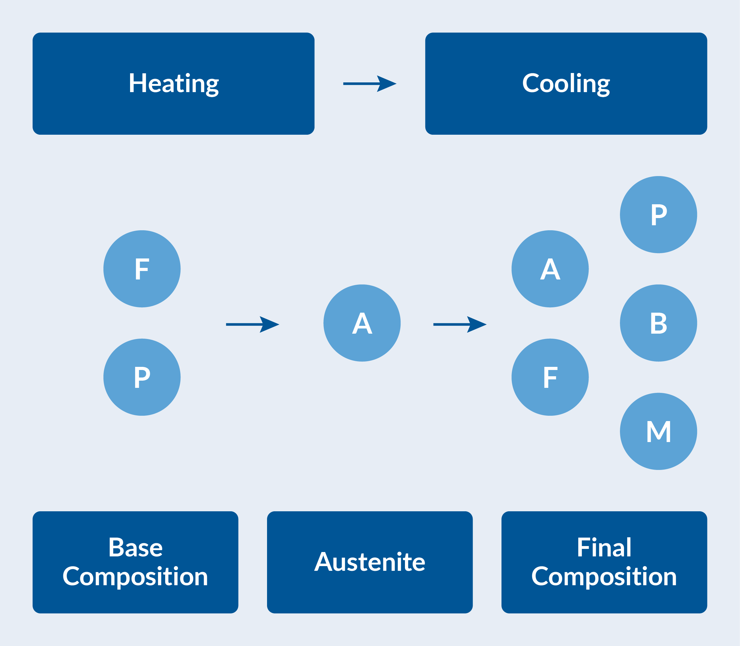
Phase composition during heating and cooling. The base composition of ferrite (F) and pearlite (P) transforms into austenite (A) on heating. The austenite decomposes into ferrite, pearlite, bainite (B), and martensite (M) during cooling.
Heating
The main purpose of simulating heating is not only to austenitize the ferritic–pearlitic steel, but also to model the thermal straining that develops on heating. Note that we could have omitted the heating part of the process by applying an initial strain at the onset of cooling to include the effect of thermal straining, but we elected to model heating prior to cooling. However, as we do not concern ourselves with the formation of austenite per se, we use the Leblond–Devaux phase transformation model to model the formation of austenite from the ferritic–pearlitic base composition. The phase transformation model uses an Additional Source Phase subnode so that both ferrite and pearlite act as source phases in the formation of austenite. The rates of the phase fractions of austenite (A), pearlite (P), and ferrite (F) are then given by:
where the equilibrium phase fraction of austenite is unity (full austenitization), and the time constant is set to 60 seconds:
Additionally, we only allow for this phase transformation during heating, and this is specified using the Transformation Condition subnode where the following condition c is entered:
audc.Tt>0
Cooling
When the fully austenitic katana is quenched in water, the austenite decomposes into a combination of ferrite, pearlite, bainite, and martensite. Depending on the rate of cooling at different locations throughout the blade, phases will form in different amounts. This suggests that more detailed descriptions of the phase transformations are required for cooling, compared to heating. The decompositions of austenite into ferrite, pearlite, and bainite are therefore modeled using the Johnson–Mehl–Avrami–Kolmogorov (JMAK) phase transformation model. This is a model that is suitable for the modeling of diffusive phase transformations. It has three parameters:
- The equilibrium phase fraction, \xi_\mathrm{eq}
- The time constant, \tau
- The Avrami exponent, n
The equilibrium phase fraction represents an equilibrium phase fraction of the destination phase that can be thought of as a long-term asymptote. For example, the equilibrium phase fraction of ferrite between the A_{e1} and A_{e3} temperatures can be evaluated by applying the lever rule to the two-phase region of austenite and ferrite in an Fe-C diagram. To determine remaining parameters, we can make use of a time–temperature-transformation (TTT) diagram. A TTT diagram typically shows when each metallurgical phase starts to form and when each transformation finishes. The TTT diagram assumes isothermal conditions, which means that if a TTT diagram is to be obtained experimentally, a test specimen should first be rapidly cooled to a “target temperature” T_\mathrm{0}, and then held at that temperature. This process is then repeated across a range of temperatures, typically ranging from the austenitization temperature, down to the temperature where martensite forms.
In the schematic below, the bottom half shows a TTT diagram where the two curves indicate the times it takes to form 1% and 99% of the destination phase. These fractions are relative phase fractions, meaning that they represent, at each temperature level, the fraction of destination phase in relation to what is maximally attainable at that temperature. The relative phase fraction is given by X =\xi^\mathrm{d}/\xi^\mathrm{d}_\mathrm{eq}, where the equilibrium phase fraction is in general, temperature dependent. Note that if these two TTT curves have been established experimentally, the JMAK phase transformation model can be fitted exactly, at each temperature. Intermediate relative phase fractions will then be dictated by the formulation of the JMAK model itself. The top half of the schematic shows the evolution of the destination phase as governed by a specific phase transformation model, at T=T_0.
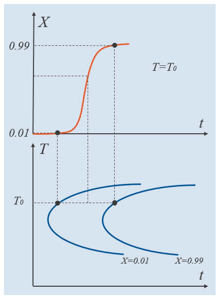
Example TTT curves for the relative phase fractions 0.01 and 0.99. An intermediate relative phase fraction is indicated.
In COMSOL Multiphysics®, the JMAK phase transformation model is expressed on rate form, making it suitable for non-isothermal conditions. In the TTT sense, however, we can integrate the JMAK model symbolically. The evolution of the destination phase with time becomes:
After some manipulation, this equation can be re-expressed as:
If we use the start and finish times and phase fractions from the figure above, assuming that the equilibrium phase fraction is known, we can identify the Avrami exponent n and the time constant \tau:
This is precisely what is done for the TTT diagram data formulation of the JMAK phase transformation model in the Phase Transformation node.
In the current model of the quenching of a katana, three sets of fictitious, but reasonable, start and finish TTT curves are used to define the decomposition of austenite into, respectively, ferrite, pearlite, and bainite. For ferrite, a section of the data is:
| T \, (^{\circ}C) | t_1 \, (s) | t_{99} \, (s) |
|---|---|---|
| 575 | 2.2 | 43 |
| 580 | 0.22 | 2.1 |
| 585 | 0.075 | 1.42 |
| 590 | 0.076 | 1.47 |
| 595 | 0.078 | 1.47 |
| 600 | 0.079 | 1.49 |
| 605 | 0.081 | 1.54 |
| 610 | 0.084 | 1.58 |
| 615 | 0.086 | 1.63 |
| 620 | 0.090 | 1.70 |
| \vdots | \vdots | \vdots |
| \vdots | \vdots | \vdots |
| 730 | 5.8 | 110 |
| 735 | 13 | 254 |
| 740 | 41 | 820 |
| 745 | 322 | 6246 |
To complete the phase transformation model definitions, we also need to identify:
- The temperature-dependent equilibrium phase fractions for ferrite, pearlite, and bainite, for the respective phase transformations.
- The upper and lower temperature limits for the phase transformation. For example, A_\mathrm{e3} defines the onset of ferritic transformation, and M_\mathrm{s} is the martensite start temperature.
The equilibrium phase fractions and the different transformation temperatures are computed based on chemical composition using the Steel Composition node under the Austenite Decomposition interface.
We only allow for these phase transformations during cooling, and just like for heating, we control this using the Transformation Condition subnode where the following condition c is entered:
audc.Tt<=0
When the TTT curves for the phase transformation into ferrite, pearlite, and bainite are used in conjunction, we can compute a TTT diagram using the Austenite Decomposition interface. The figure below shows the computed TTT diagram. To model this, we use the Austenite Decomposition interface in 0–D, and the times to reach certain phase fractions are obtained by selecting Compute transformation times in the phase nodes.
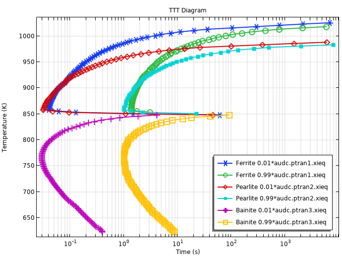
Computed TTT Diagram using the fictitious TTT data.
The martensitic phase transformation is described by the Koistinen–Marburger phase transformation model. This model requires two parameters:
- The Koistinen–Marburger coefficient, \beta
- The Martensite start temperature, M_\mathrm{s}
Unlike the diffusive ferritic, pearlitic, and bainitic transformations that were considered under isothermal conditions, the martensitic transformation is inherently temperature rate dependent. The rate at which martensite forms, according to the Koistinen–Marburger model, is proportional to the cooling rate through the coefficient \beta.
With all phase transformations defined, we can also compute a continuous cooling transformation (CCT) diagram. The figure below shows a CCT diagram, where the austenitization temperature is 900°C, and the cooling rates range from 0.1 K/s to 1000 K/s. The 1% lines are shown for the formed ferrite, pearlite, bainite, and martensite phases. The 1% line is also shown for austenite, and this can be considered the completion of the austenite decomposition — almost all austenite has decomposed into other phases.
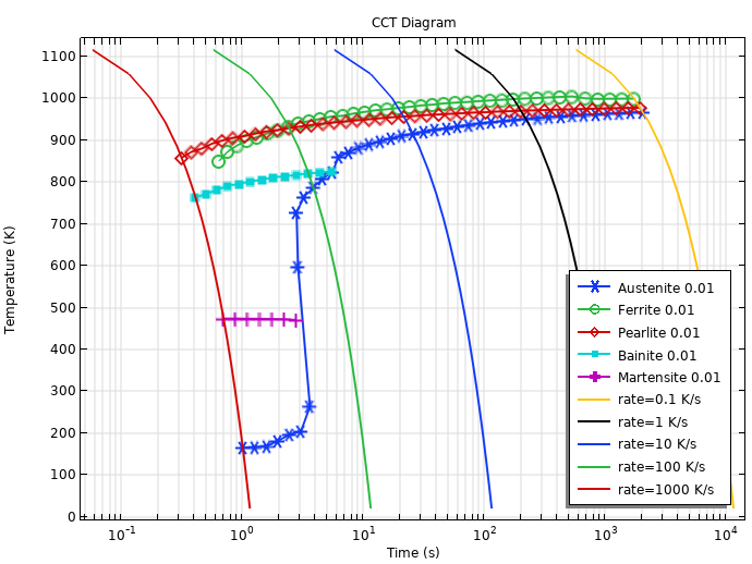
Computed CCT Diagram based on the TTT data.
Mechanical and Thermal Material Properties
For a detailed model of the quenching of a steel component such as a katana, thermal and mechanical properties are required. These properties vary between phases, such as austenite and ferrite, and moreover, they depend on temperature. For elastoplastic properties, there is generally also a dependence on strain and possibly strain rate. Obtaining a complete set of material properties experimentally is time consuming and expensive, and thus, often prohibitive. In practice, other sources are used, including experimental data from the literature and computed material properties. The purpose of the present simulation is to demonstrate the quenching of a katana, and in light of this, we make the following modeling simplifications:
- The elastic properties are shared between phases, but remaining properties are taken to vary between phases.
- The thermal conductivities and the heat capacities are taken as temperature dependent.
- The initial yield stresses are taken as temperature dependent.
- The hardening behaviors of the phases are taken as linear and isotropic, and temperature dependent.
- The thermal expansion coefficients are constant, but the volume reference temperatures vary.
The material properties for each phase, together with the evolving phase composition (phase fractions), are used to compute effective material properties. This is done automatically in the Metal Processing Module, and the computed effective properties are collected in a Compound Material for transparent use by other physics interfaces. See the figure below.
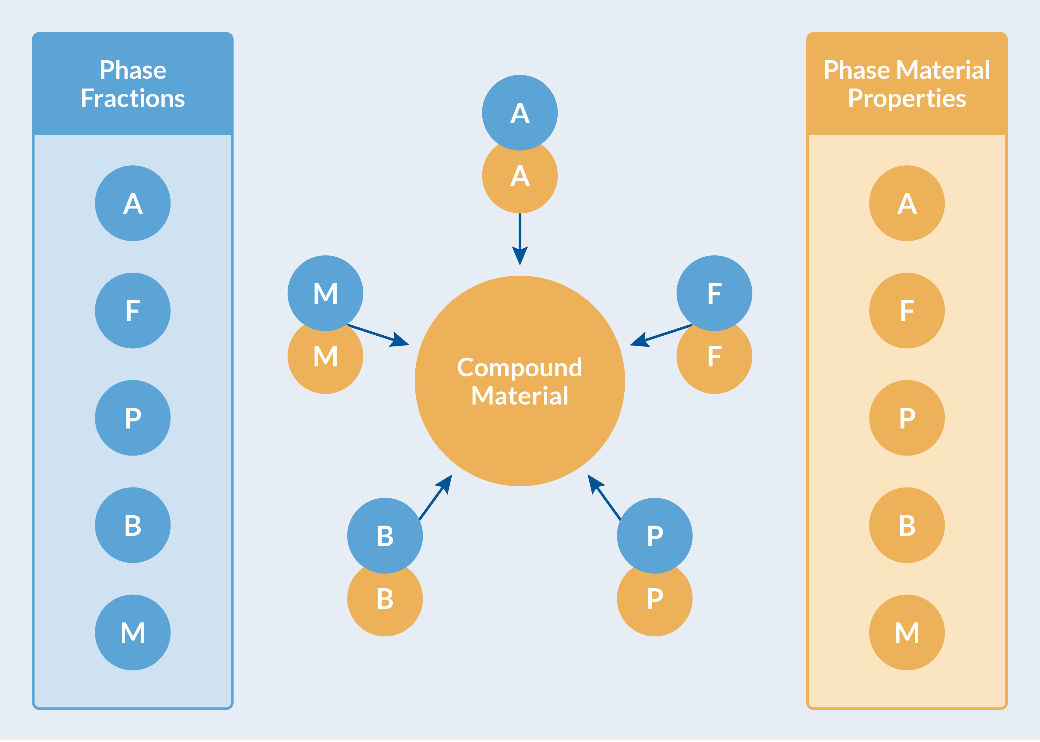
Computed effective material properties are collected in a Compound Material.
Heat Transfer Modeling
The Heat Transfer in Solids interface is used to model the heat transport in the katana and the heat exchange with the surrounding environment. For simplicity, radiation is neglected, and the heat transfer from the blade to the surrounding environment is modeled using convection alone. A heat flux is prescribed on the surface of the blade, and it is characterized by a temperature-dependent heat transfer coefficient.
Heating
The heating of the katana is done to austenitize the ferritic–pearlitic base composition. To model this, we use a simplified model for the convection using a constant heat transfer coefficient of 300 W/m^2K. The ambient temperature is ramped from room temperature to 850°C during the first minute of heating and then kept constant for the duration of the heating. The total time is chosen so that the material transforms fully into austenite, and the heating is such that thermal gradients in the katana are low enough to prevent thermally induced plastic straining.
Cooling
To emulate the effect of different thicknesses of the insulating clay, the heat transfer coefficient will be different for the region near the edge of the blade, compared to the upper part of the blade.
The figure below shows the temperature-dependent heat transfer coefficients that have been used to represent thin and thicker layers of clay.
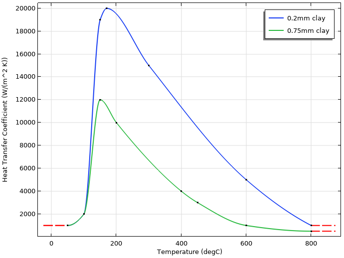
Temperature-dependent heat transfer coefficients for the thin (0.2 mm) and thicker (0.75 mm) layers of clay. The thin layer is applied to the edge, while the thicker layer is applied to the rest of the blade.
Stress and Strain Modeling
The Solid Mechanics interface is used to compute stresses, strains, and distortions of the katana during the thermal transient that it is subjected to. We pointed out earlier that thermal expansion and density differences between phases result in distortions of the component, as well as mechanical stresses and plastic strains. These effects are handled by the Austenite Decomposition interface and transferred to the Solid Mechanics interface using the Phase Transformation Strain multiphysics coupling. We anticipate significant bending of the katana. Bending of a slender structure does not necessarily produce large material strains. However, finite rotations are involved, and the analysis is therefore geometrically nonlinear. The bending is also expected to produce plastic straining, and the Plasticity subnode to Linear Elastic Material is used to account for this.
Results
One of the most notable characteristics of the katana is its curved blade. What’s interesting is that this curvature emanates from the quenching process and not from bending the blade prior to heat treating it. As the blade is thinner near the edge, where the insulating clay is also more thinly applied, the temperature drops rapidly, and the blade initially bends downwards as the austenite cools and contracts. When the temperature drops below the martensite start temperature, the austenite begins to transform into martensite. The transformation into martensite is accompanied by volumetric expansion, which causes compressive stresses at the edge of the blade. As the cooling progresses toward the ridge of the blade, the rate of cooling becomes lower and other metallurgical phases form. The initial downward bend of the blade transitions into the final, traditional curved shape of the sword. The bottom figure shows the final composition of metallurgical phases. Notably, the edge is martensitic, and thus hard, but the ridge of the blade is largely pearlitic, and as such, considerably more ductile.
Axial stress (top), equivalent plastic strain (middle), and phase fraction of martensite (bottom) at the end of the cooling.
The final composition after quenching. The edge has the desired hard martensitic structure, and the ridge of the blade is largely pearlitic.
Applying What We Learned
In this blog post, we showed how to perform a quenching simulation of a katana using COMSOL Multiphysics®. We explained how the katana got its curved shape and how a simplified version of the traditional process of using clay for differential quenching produced a blade with a hard edge and a soft core. Modeling a katana is, of course, merely a curiosity; however, it showed that COMSOL Multiphysics® can be used to perform general steel hardening simulations, in which you can compute not only the composition of metallurgical phases but also predict distortions and residual stresses.
Try It Yourself
Want to try modeling the differential quenching of a katana? The model files are available in the Application Gallery.


Comments (0)