
Engineers are given significant freedom in their pursuit of lightweight structural components in airplanes and space applications, so it makes sense to use methods that can exploit this freedom, making topology optimization a popular choice in the early design phase. This method often requires regularization and special interpolation functions to get meaningful designs, which can be a nuisance to both new and experienced simulation users. To simplify the solution of topology optimization problems, the COMSOL® software contains a density topology feature.
About the Density Method for Topology Optimization
As the name suggests, topology optimization is a method that has the ability to come up with new and better topologies for an engineering structure given an objective function and set of constraints. The method comes up with these new topologies by introducing a set of design variables that describe the presence, or absence, of material within the design space. These variables are defined either within every element of the mesh or on every node point of the mesh. Changing these design variables thus becomes analogous to changing the topology. This means that holes in the structure can appear, disappear, and merge as well as that boundaries can take on arbitrary shapes. In addition, the control parameters are somewhat automatically defined and tied to the discretization.
As of COMSOL Multiphysics® software version 5.4, the add-on Optimization Module includes a density topology feature to improve the usability of topology optimization. The feature is designed to be used as a density method (Ref. 3), meaning that the control parameters change a material parameter through an interpolation function. Interpolation functions for solid and fluid mechanics are built into the feature and used in example models throughout the Application Library in COMSOL Multiphysics.

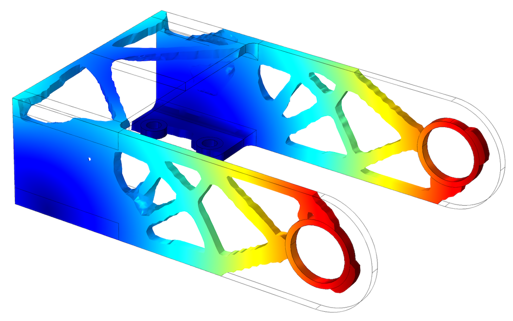
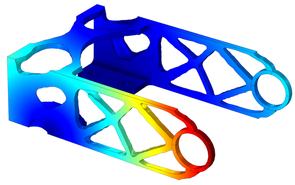
A bracket geometry is topology optimized, leaving only 50% of the material, which contributes the most to the stiffness.
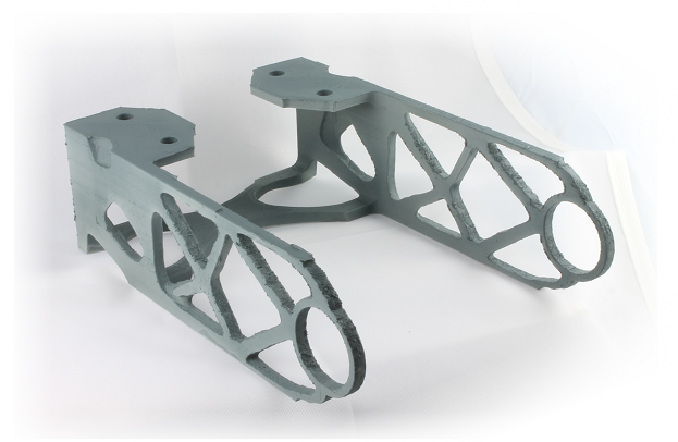
The printed bracket geometry.
The density method involves the definition of a control variable field, \theta_c, which is bounded between 0 and 1. In solid mechanics, \theta_c=1 corresponds to the material from which the structure is to be built, while \theta_c=0 corresponds to a very soft material. By default, the void Young’s modulus is 0.1% of the solid Young’s modulus. In fluid mechanics, convention dictates that \theta_c=1 corresponds to fluid, while \theta_c=0 is a (slightly) permeable material with an inverse permeability factor, \alpha; i.e., a damping term is added to the Navier-Stokes equation:
The damping term is 0 in fluid domains, while a large value is used in solid domains. These different values give a good approximation of the no-slip boundary condition on the interface between the domains.
An Introduction to the Density Model Feature
The Density Model feature supports regularization via a Helmholtz equation (Ref. 1). This introduces a minimum length scale using the filter radius, R_\mathrm{min}:
Here, \theta_c is the raw control variable, which is modified by the optimizer, and \theta_f is the filtered variable. The mesh edge size is the default value for the filter radius. While this works well in terms of regularizing the optimization problem, it’s important to set a fixed length (larger than the mesh edge size) to get mesh-independent results.
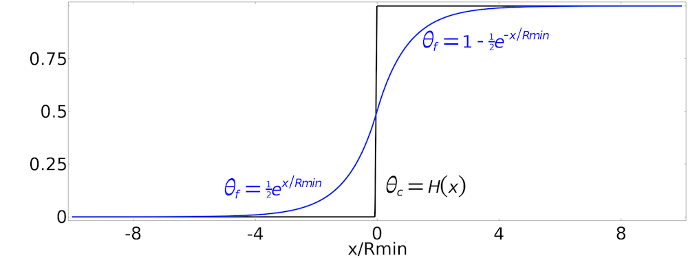

Top: The equation for the Helmholtz filter can be solved analytically for a 1D Heaviside function. Bottom: This plot is taken from the MBB beam optimization model. It shows the raw control variables to the left and the filtered version to the right.
The Helmholtz filter gives rise to significant grayscale, which does not have a clear physical interpretation. The grayscale can be reduced by applying a smooth step function in what is referred to as projection in topology optimization. Projection reduces grayscale, but it also makes it more difficult for the optimizer to converge. The density topology feature supports projection based on the hyperbolic tangent function, and the amount of projection can be controlled with the projection steepness, \beta.
Here, \theta_{\beta} is the projection point.

Plot showing the filtered field to the left and the projected field to the right.
Projection makes it possible to avoid grayscale, but grayscale can still appear if the optimization problem favors it. If the same interpolation function is used for the mass and the stiffness, grayscale is optimal in volume-constrained minimum compliance problems. It is thus common to use interpolation functions that cause intermediate values to be associated with little stiffness relative to their cost (compared to the fully solid value). You can think of this as a penalization of intermediate values for the material volume factor, and the Density Model interface (shown below) supports two such interpolation schemes for solid mechanics: solid isotropic material with penalization (SIMP) and rational approximation of material properties method (RAMP) interpolation. Darcy interpolation is provided for fluid mechanics. The interpolated variable is called the penalized material volume factor, \theta_p, and is used for interpolating the material parameters, e.g., for SIMP interpolation, the p_\textsc{simp} exponent can be increased to reduce the stiffness of intermediate values, so that grayscale becomes less favorable.
\theta_p %26= \theta_\mathrm{min}+(1-\theta_\mathrm{min})\theta^{p_\textsc{simp}}\\
E_p %26= E\theta_p
\end{align}
Here, E is the Young’s modulus of the solid material and E_p is the penalized Young’s modulus to be used throughout all optimized domains.
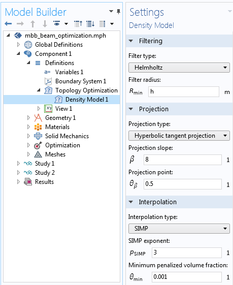
The Density Model feature is available under Topology Optimization in Component > Definitions. The mesh edge length is taken as the default filter radius and it works well, but it has to be replaced with a fixed value in order to produce mesh-independent results.
The penalized Young’s modulus can be defined as a domain variable, or (as in the case of the bracket model) it can be defined directly in the materials.
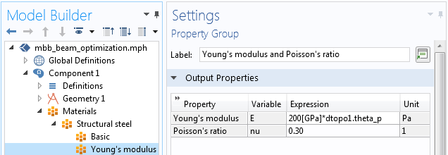
Topology optimization with the density method involves varying the Young’s modulus spatially. In this case, it is achieved by going to the material properties and multiplying the solid Young’s modulus with the penalized material volume factor, dtopo1.theta_p.
In summary, the density topology feature adds four variables. The filtered material volume factor is defined implicitly using a dependent variable.
| Symbol | Description | Equation |
|---|---|---|
| \theta_c | Control material volume factor | 0\leq\theta_c\leq1 |
| \theta_f | Filtered material volume factor | \theta_f = R_\mathrm{min}^2\mathbf{\nabla}^2\theta_f + \theta_c |
| \theta | Material volume factor | \theta = \frac{\tanh(\beta(\theta_f-\theta_{\beta}))+\tanh(\beta\theta_{\beta})}{\tanh(\beta(1-\theta_{\beta}))+\tanh(\beta\theta_{\beta})} |
| \theta_p | Penalized material volume factor | \theta_p = \theta_\mathrm{min}+(1-\theta_\mathrm{min})\theta^{p_\textsc{simp}} or \theta_p = \frac{q_\mathrm{Darcy}(1-\theta)}{q_\mathrm{Darcy}+\theta} |
When the filtering is disabled, the filtered variable becomes undefined and the projection instead uses the control material volume factor directly. If the projection is disabled, the material volume factor still exists, but it becomes identical to the projection input.
Applying Continuation to Avoid Local Minima
When the topology is not too complicated, the default values of the density topology feature work well. This is the case for the MBB beam optimization and topology optimized hook models. If the optimal design is more complicated (such as for the bracket example shown at the top of this post), there might be many local minima. To avoid these minima, you can use continuation in the SIMP exponent and the projection slope. This can be achieved by modifying the initial value expression in the density topology feature and adding a Parametric Sweep feature, as shown below. As a result, the solver ramps over the specified parameters, using the optimum from the previous case as the initial value for the next optimization step. That is, it starts with a small SIMP exponent and projection slope and then continues to higher values.
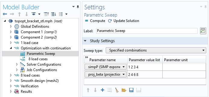
It is possible to apply continuation by combining a parametric sweep with a study reference. See the Bracket — Topology Optimization tutorial model for details.
Objectives and Constraints in Topology Optimization
If the geometry is optimized for a single load case (as shown below to the left), the resulting design will be optimal with respect to that load case. This can seem obvious, but often designers make assumptions about symmetries and the design topology. Unless these assumptions are formalized as constraints, they will not be respected. Therefore, the design shown to the right below uses eight load cases (two load groups times four constraint groups).
Left: The bracket geometry is optimized for a single load case, resulting in an asymmetric design with two loosely connected halves. Right: The bracket geometry with eight load cases.
Designers often have several objectives that need to be weighted. To make an informed decision about these objectives, a designer can trace the Pareto optimal front using several optimizations with different weights.
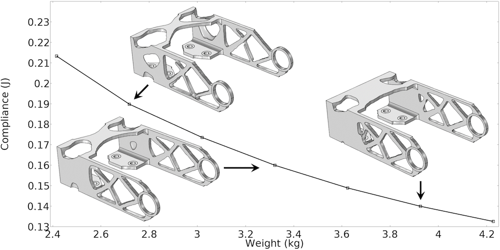
The Pareto optimal front for the bracket geometry can be traced by varying the weight in a parametric sweep.
Animation of the topology optimized bracket. (Download the glTF™ file from the Application Gallery in GLB-file format to rotate the geometry yourself.)
Exporting and Importing Topology Optimization Results
It is possible to analyze the result of a topology optimized design with respect to stress concentration and buckling without remeshing. However, if you want to be completely sure that the void phase does not play a role, you can eliminate it by exporting and importing the resulting design, as shown below. The details of this procedure are discussed in a previous blog post.
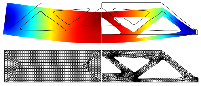
The contour (left) for the topology optimized MBB beam design is exported and imported as an interpolation curve (right).
Next Steps
To learn more about the built-in tools and features for solving optimization problems, check out the Optimization Module product page by clicking the button below.
Further Resources
- Try using the density feature for topology optimization with these example models:
- Read more about topology optimization on the COMSOL Blog:
References
- B.S. Lazarov and O. Sigmund, “Filters in topology optimization based on Helmholtz‐type differential equations,” International Journal for Numerical Methods in Engineering, vol. 86, no. 6, pp. 765–781, 2011.
- F. Wang, B.S. Lazarov, and O. Sigmund, “On projection methods, convergence and robust formulations in topology optimization,” Structural and Multidisciplinary Optimization, vol. 43, pp. 767–784, 2011.
- M.P. Bendsøe, “Optimal shape design as a material distribution problem,” Structural Optimization, vol. 1, pp. 193–202, 1989.
glTF and the glTF logo are trademarks of the Khronos Group Inc.



Comments (19)
Abdullah Shaikh
December 13, 2020Hi Kristian,
I am a student and am using COMSOL for the first time. I want to use COMSOL topology optimization to create a custom torque sensor (in other words an elastic element or a flat torsional spring) with a specified target stiffness 900Nm/rad. The design space is limited by the outer and inner boundaries and a torque (100Nm) is applied through the shaft and i want the elastic element to show linear angular deflection when torque ranges from 0 to 100 Nm.
I am an undergrad student and recently exposed to topology optimization so i would like to know exactly how i can make such an element using COMSOL if it is possible in the first place? Thanks
Kristian Ejlebjærg Jensen
December 14, 2020 COMSOL EmployeeHi Abdullah
I guess you want to include geometric nonlinearity. We can do this, but you might want to add some more objectives/constraints for topology optimization to make the problem more well-posed. Shape optimization might be a better fit in this case.
I recommend that you contact comsol.com/support, if you need help with the setup of a specific model.
best regards,
Kristian E. Jensen
Technical Product Manager, Optimization
Andrew Bayba
June 17, 2021Hi Kristian,
I am rather new to Comsol, and especially Topology Optimization. I would like to perform two-material TO on a thermal problem (Solids only, time dependent). I have a functional 2D single material TO model using the density method; now I’d like to expand that to a multi-material model (without voids). Is there a simple way to do this?
Thanks,
Andy
Kristian Ejlebjærg Jensen
June 18, 2021 COMSOL EmployeeHi Andrew
If you are new to topology optimization and COMSOL, you should try to do simple stationary one-material TO first. Then you can look at using two density models to achieve two-material TO. Finally, you can proceed to optimization on a time dependent problem. The individual steps are not complicated, but you save time and reduce risk of project failure, if you avoid going for time dependent two-material TO right away.
best regards,
Kristian E. Jensen
Technical Product Manager, Optimization
Andrew Bayba
June 22, 2021Kristian,
Yes, I have performed a fair amount of work on a relatively simple single material model with and without time dependency, and am now “very interested” in moving on to 2 materials.
Andy
Alex Angilella
September 16, 2022The theta_p equation does not agree with the COMSOL documentation. I think the first variable is supposed to be added to the other multiplied terms.
Kristian Ejlebjærg Jensen
September 16, 2022 COMSOL EmployeeThank you for pointing this out. The theta_p equation is correct in COMSOL, in the documentation and in the table of this blog post, but there is indeed a “+” missing in the first equation for theta_p in this blog post.
Haiyang Li
December 16, 2022I have 2 questions
1. theta is the projected variable, why don’t called it projected material volume factor
2. In this statement
If the projection is disabled, the material volume factor still exists, but it becomes identical to the projection input.
I wonder what is the projection input? Is it theta_beta, the projection point?
Kristian Ejlebjærg Jensen
December 16, 2022 COMSOL Employee1. Theta is the input to the interpolation/penalization. It would be strange to call it projected material volume factor, because projection can be disabled.
2. Yes theta_beta is the projection point.
Haiyang Li
December 16, 2022In the Penalized material volume factor theta_p, there’s theta_min, I saw in the reference of “Topology Optimization of an MBB Beam” that theta_min is called relative minimum Young’s modulus. I don’t understand why it is called Young’s modulus? Because I think E(x) or E_0 is something related to Young modulus?
Haiyang Li
December 17, 2022Hi Kristian,
I’m confused with the sequence of TO, it is
1. Penalization
2. Filtering
3. Projection
or
1. Filtering
2. Projection
3. Penalization?
Kristian Ejlebjærg Jensen
December 17, 2022 COMSOL EmployeeIt is the latter ordering, same as the order of the sections in the GUI of the feature. You are right, that it would be more consistent to use “minimum penalized volume fraction” in the documentation of the mbb_beam_optimization model.
Manal Shlebik
March 16, 2023Hi Kristian,
Thank you for the clarification and useful information,
I want to use COMSOL topology optimization to create holes inside the device,
I am following your steps but using Wave optics instead of Solid Mechanics. My goal is to create holes to reduce the material and maximize the transmission of Electromagnetic waves at the desired frequency. Therefore, I think my objective function should be Total transmittance.
Your Objective function is: Total elastic strain energy to increase the stiffness
Your constraint is: Average material volume factor= 0.5 to reduce 50 % of the amount of material.
Would “Total transmittance (comp1.ewfd.Ttotal)” be suitable to be introduced as the expression for the objective function to achieve my goal, please?
I want to reduce 50% of the material, Would my constraint be ok to be written the same as yours, please?
Thanks in advance,
Manal
Kristian Ejlebjærg Jensen
March 16, 2023 COMSOL EmployeeHi Manal
We do not have examples of topology optimization with wave optics, but it has been done before with COMSOL. However, local minima is a common problem for topology optimization of wave propagation problems. Have you considered doing shape optimization instead? We recently published a blog post on shape optimization for wave optics applications: https://www.comsol.com/blogs/shape-optimization-in-electromagnetics-part-1/
Manal Shlebik
March 16, 2023Hi Kristian,
Thank you for your response,
Yes, I have followed your example: waveguide_filter_optimization_polynomial using shape optimization. I have involved the same objective function and control variables: Polynomial Boundary. However, I could not reach my target which is to maximize the transmission of Electromagnetic waves at the desired frequency through a 3D power splitter, I need to create holes inside the device. Also, I got the error message saying:
(MUMPS is switching to out-of-core mode)
Would you please help me to achieve this?
Best regards,
Manal
Kristian Ejlebjærg Jensen
March 16, 2023 COMSOL EmployeeHi Manal, I suggest that you contact comsol.com/support
Haiyang Li
February 29, 2024In this example: https://www.comsol.com/model/topology-optimization-of-an-mbb-beam-7428
It adopted 2 times of interpolation with different design variables theta and theta_p.
1. Interpolate the density using theta (the design variable after projection):
rho = theta rho_0
2. Interpolate the material property (Young’s modulus) using theta_p:
theta_p = theta_min + (1 + theta_min) theta^n
E_SIMP = theta_p E
As shown follows
Density rho root.comp1.dtopo1.theta*(7850[kg/m^3]) kg/m³ Basic
Young’s modulus E root.comp1.dtopo1.theta_p*(E(T)) Pa Young’s modulus and Poisson’s ratio
Why do we interpolate the density using theta?
Haiyang Li
February 29, 2024In this example: “https://www.comsol.com/model/topology-optimization-of-an-mbb-beam-7428“
It adopted 2 times of interpolation with different design variables theta and theta_p.
1. Interpolate the density using theta (the design variable after projection):
rho = theta rho_0
2. Interpolate the material property (Young’s modulus) using theta_p:
theta_p = theta_min + (1 + theta_min) theta^n
E_SIMP = theta_p E
As shown follows
Density rho root.comp1.dtopo1.theta*(7850[kg/m^3]) kg/m³ Basic
Young’s modulus E root.comp1.dtopo1.theta_p*(E(T)) Pa Young’s modulus and Poisson’s ratio
Why do we interpolate the density using theta?
Kristian Ejlebjærg Jensen
March 1, 2024 COMSOL Employee“If the same interpolation function is used for the mass and the stiffness, grayscale is optimal in volume-constrained minimum compliance problems.”