Postprocessing Local Data Using Component Coupling

Component coupling operators are a useful set of tools included in COMSOL Multiphysics. They can be used to derive numerical values, create new coordinate systems, and link different components in the same model. In this blog post, we will explore yet another possibility: Using General Extrusion, one of the component coupling operators, to extract local solution data and postprocess effectively.

A Postprocessing Challenge

After obtaining a solution, we often want to zoom in and take a closer look at a smaller region. For example, after we run an analysis for the structural mechanics of a loaded spring, we may want to not only visualize the solved variables on the entire spring, but also plot the data in some local regions. The figure below shows such an area along the midplane of the curved geometry.

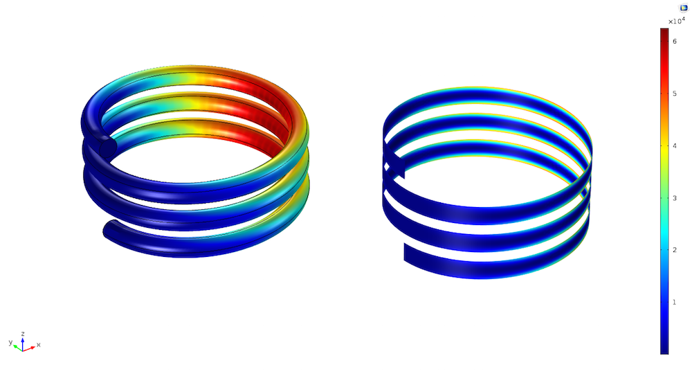
Elastic strain energy density of a loaded spring plotted on all surfaces (left) versus on a vertical midplane (right). Note that this midplane does not exist in the original geometry when the structural mechanics analysis is performed.

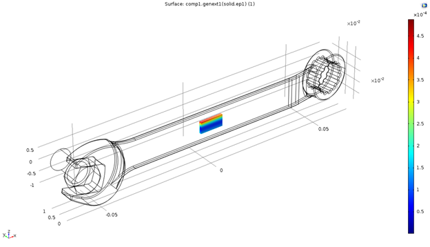
Another example is when we are interested in visualizing data in a particular 3D shape that does not exist in the original model. This comes after performing a structural mechanics analysis of a wrench. See the figure below.

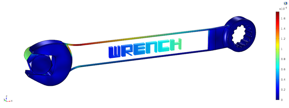
First principal strain of a wrench plotted on an arbitrary 3D domain. Again, the 3D domain does not exist in the original geometry.

If this region of interest is an existing, separate geometry domain, then the data extraction and visualization can be easily done via a selection of that domain. However, we do not usually know where to look before seeing the results, and it could be difficult to partition the whole geometry into separate domains a priori. On the other hand, once we have solved the physics, it is impractical to modify the geometry, mesh, and solve the model all over again only for postprocessing purposes. How should we deal with this challenge?

A Practical Approach to Postprocessing Local Data

One of the component coupling operators, General Extrusion, gives us the solution. The key idea is to build the region of interest as a new geometry in a new component and then use the General Extrusion operator to map the solution data from the original component onto this new component. This approach avoids remeshing and re-solving of the original component. Another advantage is that the new component can be of arbitrary shape (but not larger than the original component) and space dimension (i.e., equal to or lower than that of the original component).

For a step-by-step tutorial to postprocessing local data, we will use the wrench tutorial model as an example, also found via File > Application Libraries > COMSOL Multiphysics > Structural Mechanics. Following the steps below, you will be able to quickly master this trick.

1. Create a General Extrusion operator in the existing component, Component 1 > Definitions. Select All domains as its source.
   
   
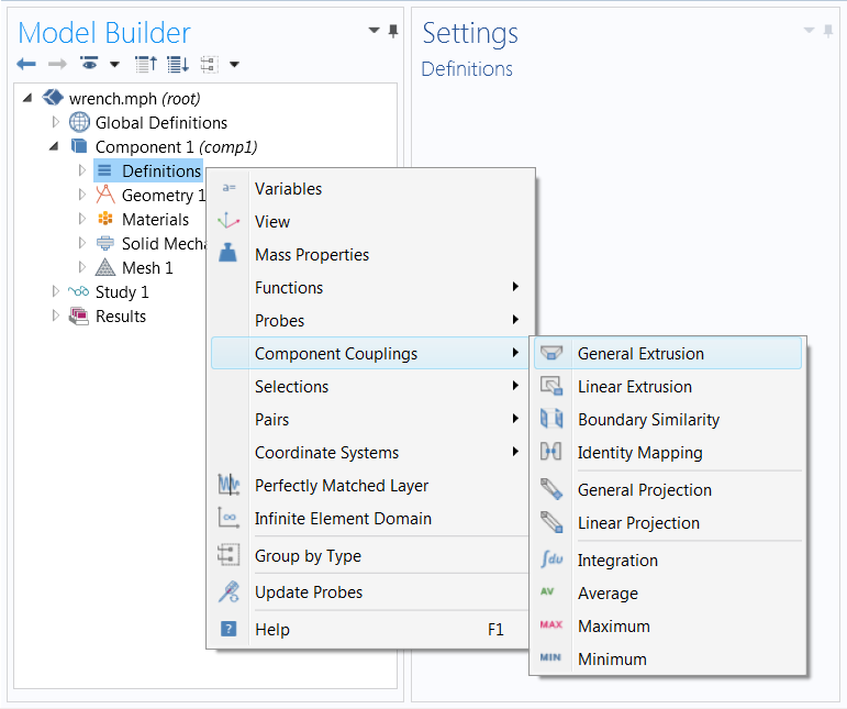
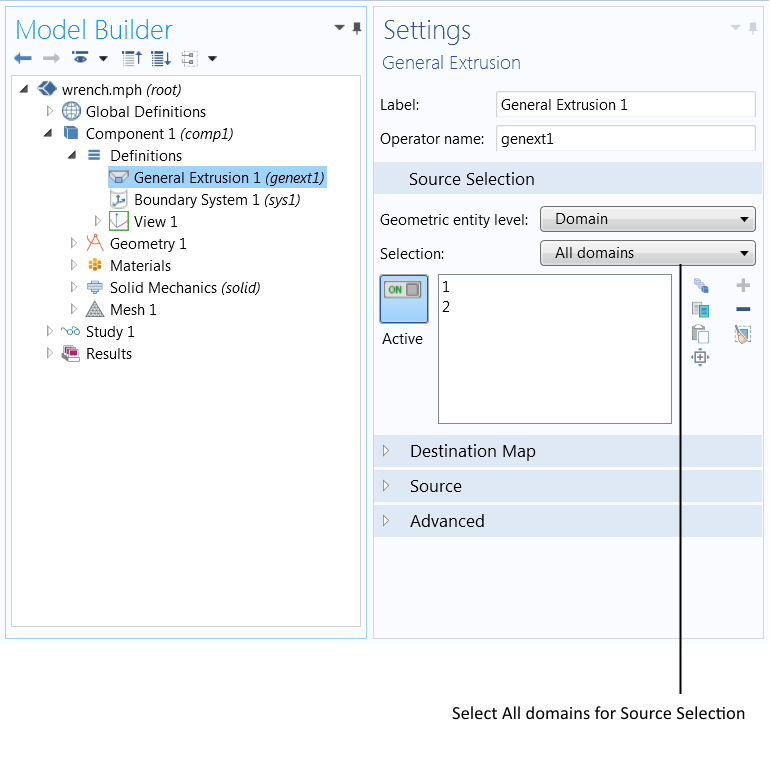
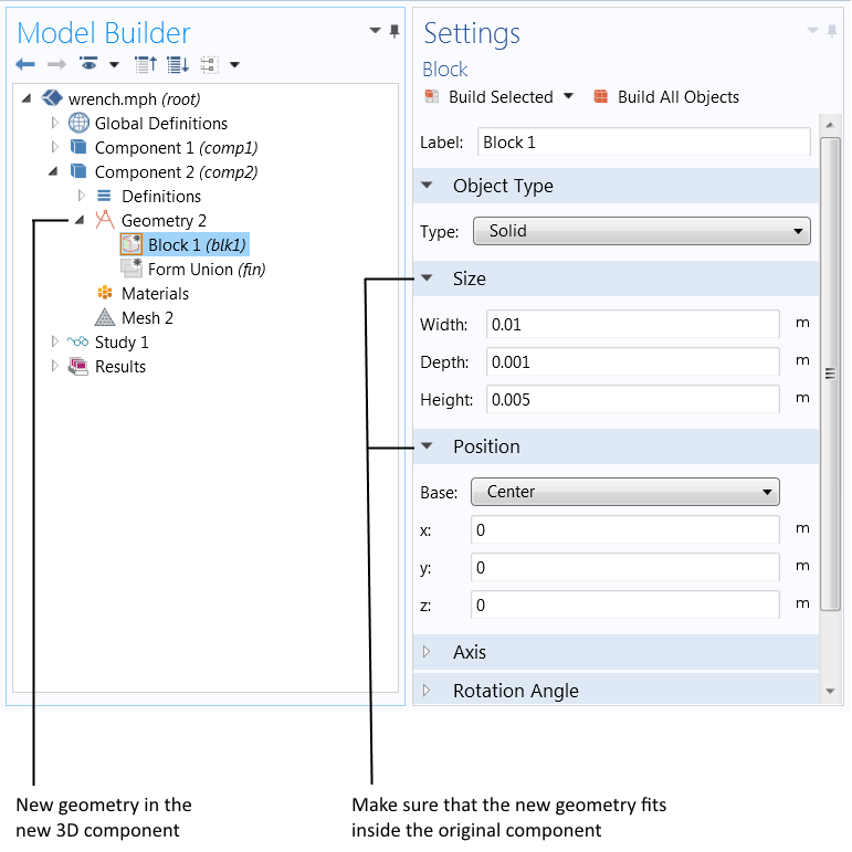
2. Create a new component in the model tree. Note that the new component must have the same or lower space dimension than the original component. Next, build the new geometry according to the way you want to extract data. Make sure that the new geometry fits inside the original component.
   
   
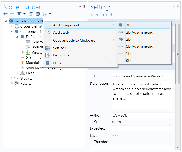
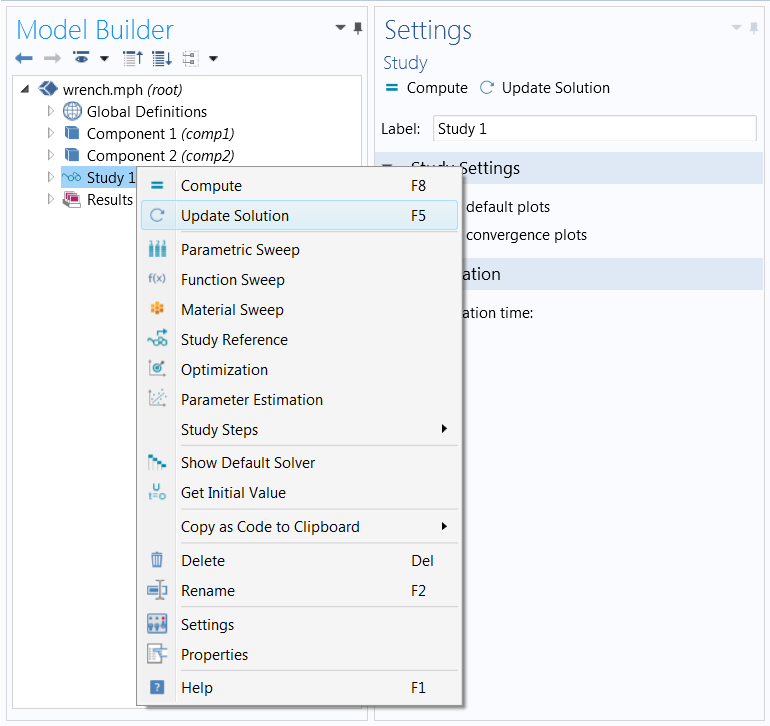
3. Right-click on the Study node and select Update Solution. This step ensures that the solution data becomes accessible in the new component.
   
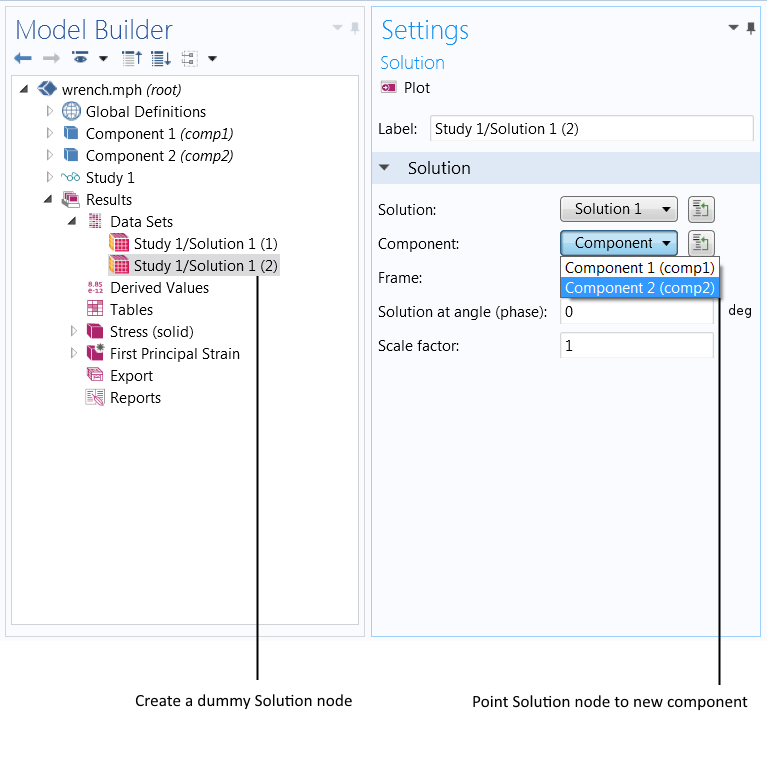
4. Create a dummy Solution node in Results > Data Sets and point this solution to the new component, Component 2 in this case.
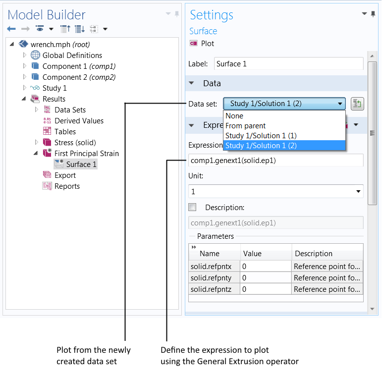
5. It’s time to plot the data. Remember to plot from the newly created data set and define the expression using the General Extrusion operator we defined earlier, comp1.genext1. This means that the plot will show results on the geometry of Component 2 (the block), using the results extruded from the study on Component 1 (the wrench). For example, solid.ep1 stands for the first principal strain in Component 1. To extrude the first principal strain from Component 1 to Component 2, we need to type comp1.genext1(solid.ep1) in the Expression input field instead.
   
   

Concluding Remarks

COMSOL Multiphysics is an extremely flexible software platform. Besides what is discussed in this blog post, you can use component couplings to perform submodeling, implement a controller, and perform model rotation. Meanwhile, the COMSOL support team would be more than happy to assist you as you explore even more possibilities.