Self-Consistent Schrödinger-Poisson Results for a Nanowire Benchmark

The Schrödinger-Poisson Equation multiphysics interface simulates systems with quantum-confined charge carriers, such as quantum wells, wires, and dots. Here, we examine a benchmark model of a GaAs nanowire to demonstrate how to use this feature in the Semiconductor Module, an add-on product to the COMSOL Multiphysics® software.

The Schrödinger-Poisson Equation Multiphysics Interface

The Schrödinger-Poisson Equation multiphysics interface, available as of COMSOL Multiphysics® version 5.4, creates a bidirectional coupling between the Electrostatics interface and the Schrödinger Equation interface to model charge carriers in quantum-confined systems. The electric potential from the electrostatics contributes to the potential energy term in the Schrödinger equation. A statistically weighted sum of the probability densities from the eigenstates of the Schrödinger equation contributes to the space charge density in the electrostatics. All spatial dimensions (1D, 1D axial symmetry, 2D, 2D axial symmetry, and 3D) are supported.

Solving the Schrödinger-Poisson System

The Schrödinger-Poisson system is special in that a stationary study is necessary for the electostatics, and an eigenvalue study is necessary for the Schrödinger equation. To solve the two-way coupled system, the Schrödinger equation and Poisson’s equation are solved iteratively until a self-consistent solution is obtained. The iterative procedure consists of the following steps:

Step 1

To provide a good initial condition for the iterations, we solve Poisson’s equation

(1)

for the electric potential, V, in which \epsilon is the permittivity and \rho is the space charge density.

In this initialization step, \rho is given by the best initial estimate from physical arguments; for example, using the Thomas-Fermi approximation.

Step 2

The electric potential, V, from the previous step contributes to the potential energy term, V_e, in the Schrödinger equation

(2)

where q is the charge of the carrier particle, which is given by

(3)

where z_q is the charge number and e is the elementary charge.

Step 3

With the updated potential energy term given by Eq. 2, the Schrödinger equation is solved, producing a set of eigenenergies, E_i, and a corresponding set of normalized wave functions, \Psi_i.

Step 4

The particle density profile, n_\mathrm{sum}, is computed using a statistically weighted sum of the probability densities

(4)

where the weight, N_i, is given by integrating the Fermi-Dirac distribution for the out-of-plane continuum states (thus depending on the spatial dimension of the model).

(5)

(6)

(7)

where g_i is the valley degeneracy factor, E_f is the Fermi level, k_B is the Boltzmann constant, T is the absolute temperature, m_d is the density of state effective mass, and F_0 and F_{-1/2} are Fermi-Dirac integrals.

For simplicity, the weighted sum in Eq. 4 shows only one index, i, for the summation. There can be, of course, more than one index in the summation. For example, in the nanowire model discussed here, the summation is over both the azimuthal quantum number and the eigenenergy levels (for each azimuthal quantum number).

Step 5

Given the particle density profile, n_\mathrm{sum}, we reestimate the space charge density, \rho , and then re-solve Poisson’s equation to obtain a new electric potential profile, V. The straightforward formula for the new space charge density

(8)

almost always leads to divergence of the iterations. A much better estimate is given by

(9)

where V_\mathrm{old} is the electric potential from the previous iteration and \alpha is an additional tuning parameter. Eq. 9 is used by the solver sequence to compute the space charge density, \rho.

The formula is motivated by the observation that the particle density, n_\mathrm{sum}, is the result from V_\mathrm{old} and would change once Poisson’s equation is re-solved to obtain a new V. In other words, Eq. 8 can be written more explicitly as

(10)

since n_\mathrm{sum} is the result from V_\mathrm{old}, and \rho is used to re-solve Poisson’s equation to get a new V.

To achieve a self-consistent solution, a better formula would be

(11)

At this point, n_\mathrm{sum,new} is unknown to us, since it comes from the solution to the Schrödinger equation in the next iteration. However, we can formulate a prediction for it using Boltzmann statistics, which provides a simple exponential relation between the potential energy, V_e=qV, and the particle density, n_\mathrm{sum}.

(12)

This leads to Eq. 9 for the case of \alpha=0. This works well at high temperatures, where Boltzmann statistics is a good approximation. At lower temperatures, setting \alpha to a positive number helps accelerate convergence.

Step 6

Once a new electric potential profile, V, is obtained by re-solving Poisson’s equation, compare it with the electric potential from the previous iteration, V_\mathrm{old}. If the two profiles agree within the desired tolerance, then self-consistency is achieved; otherwise, go to step 2 to continue the iteration.

A dedicated Schrödinger-Poisson study type is available to automatically generate the steps outlined above in the solver sequence.

Benchmark Example: The Nanowire Model

The GaAs nanowire tutorial model is based on a paper by J.H. Luscombe, A.M. Bouchard, and M. Luban titled “Electron confinement in quantum nanostructures: Self-consistent Poisson-Schrödinger theory”.

Given the assumption of an infinite length and cylindrical symmetry, we choose the 1D axisymmetric space dimension. We then select the Schrödinger-Poisson Equation multiphysics interface under the Semiconductor branch, which adds the Schrödinger Equation and Electrostatics interfaces together with the Schrödinger-Poisson Coupling multiphysics coupling in the Model Builder.

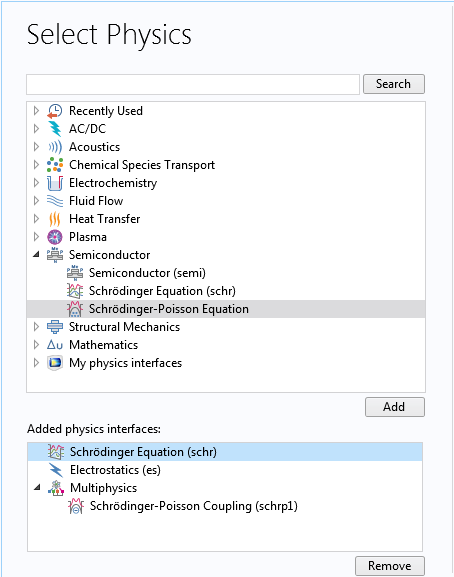
Selecting the Schrödinger-Poisson Equation interface for the nanowire model.

Following the description in the paper, the radius of the nanowire is set to 50 nm. The electron effective mass is set to 0.067 times the free electron mass (as suggested by the Fermi-temperature result in the paper), and the dielectric constant is assumed to be 12.9. The Fermi energy level in the model is set to 0 V and the electric potential at the wall to −0.7 V in order to match the Fermi-level-pinning boundary condition described by the researchers. We model the case of 2·10¹⁸ cm^–3 uniform ionized dopants at a temperature of 10 K to compare with Figures 2 and 3 in the paper. The numbers above are entered as global parameters in the model.

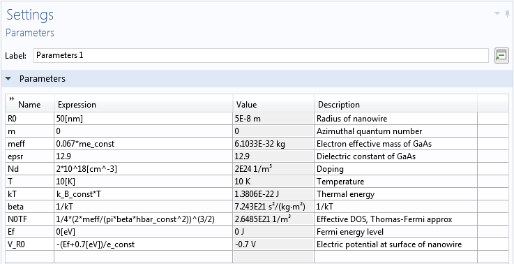
Global parameters for the nanowire model.

Following the approach of the paper, we first solve for the Thomas-Fermi approximate solution, then use it as the initial condition for the fully coupled Schrödinger-Poisson equation. The formulas for the Thomas-Fermi approximation are entered as local variables in the model.

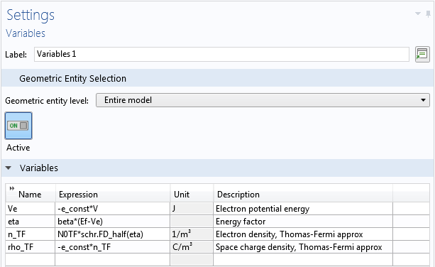
Local variables for the nanowire model.

With the global parameters and local variables defined, it is straightforward to use them to fill the various input fields in the geometry, material, and physics nodes in the Model Builder. Here are a few things to note:

• The azimuthal quantum number m is parameterized to allow sweeping and summing over its values, as mentioned above, and is entered in the Settings window of the Schrödinger Equation physics node
• Recall from a previous blog post on computing the band gap for superlattices that the eigenvalue scale λ_scale works as a multiplication factor for the dimensionless eigenvalue λ to produce the eigenenergy, E_i (E_i = λ_scale λ)
  • For instance, if λ_scale equals 1 eV, then an eigenvalue of 1.23 indicates an eigenenergy of 1.23 eV
• For the Electrostatics interface, an Electric Potential boundary condition is added to set the value at the wall of the nanowire, as mentioned above
• In addition, two Space Charge Density domain conditions are added, one for the ionized dopants and the other for the Thomas-Fermi approximation (the latter should be turned off for the Schrödinger-Poisson study)

Setting Up the Schrödinger-Poisson Multiphysics Coupling

In the Settings window for the Schrödinger-Poisson Coupling multiphysics node, expand the Equation section to see the equations implemented in this node — they should look familiar if you’ve read the Solving the Schrödinger-Poisson System section above. The Coupled Interfaces section in the settings allows the selection of the two coupled physics interfaces. The Model Input section sets the temperature of the system, as shown in the screenshot below:

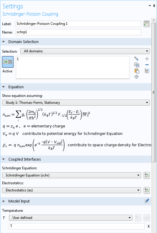
Upper part of the Settings window for the Schrödinger-Poisson Coupling node.

The Particle Density Computation section (screenshot below) specifies the statistically weighted sum of the probability densities, as described in Eq. 4. If the default option of Fermi-Dirac statistics, parabolic band is selected, then Eq. 5–Eq.7 are used to compute the weights, N_i. A user-defined option is also available for entering different expressions for the weights.

To take into account the pairs of degenerate azimuthal quantum numbers (m = ±1, ±2, etc.), we use the formula 1+(m>0) for the Degeneracy factor, g_i, which evaluates to 1 for m = 0 and 2 for m > 0.

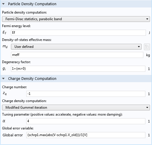
Lower part of the Settings window for the Schrödinger-Poisson Coupling node.

The Charge Density Computation section (screenshot above) takes the input for the Charge number, z_q, for Eq. 3. If the default option of Modified Gummel iteration is selected, then Eq. 9 is used to compute the new space charge density, \rho. Other options are also available, including a user-defined option where you can enter your own mathematical expressions.

The default expression for the Global error variable, (schrp1.max(abs(V-schrp1.V_old)))/1[V], computes the maximum difference between the electric potential fields from the two most recent iterations, in the unit of V. Note that the prefix schrp1 should match the Name input field of the Schrödinger-Poisson Coupling node, and the variable name V should match the dependent variable name for the Electrostatics interface. These names may change from the default in a more complicated model, and the expression will turn yellow if the names do not match. In this case, some manual editing is needed.

Setting Up the Schrödinger-Poisson Study Step

The dedicated Schrödinger-Poisson study step under Study 2 automatically generates the self-consistent iterations in the solver sequence. The iteration scheme is outlined in Solving the Schrödinger-Poisson System above.

If we are dealing with a completely new problem, then for the Eigenfrequency search method menu under the Study Settings section, it is often necessary to use the default Manual search option to find the range of the eigenenergies. Once the range is found, we can switch to the Region search option with appropriate settings for the range and number of eigenvalues in order to ensure that all significant eigenstates are found by the solver. For this tutorial, the estimated energy range is between -0.15 and 0.05 eV. This corresponds to -0.15 and 0.05 for the unitless eigenvalue, as discussed earlier.

The real and imaginary parts of the input fields refer to the real and imaginary parts of the eigenvalue, respectively. To look for the eigenenergies of bound states, we set the input fields for the real parts to the expected energy range and set the input fields for the imaginary parts to a small range around 0 to capture numerical noise or slightly leaky quasibound states, as shown below:

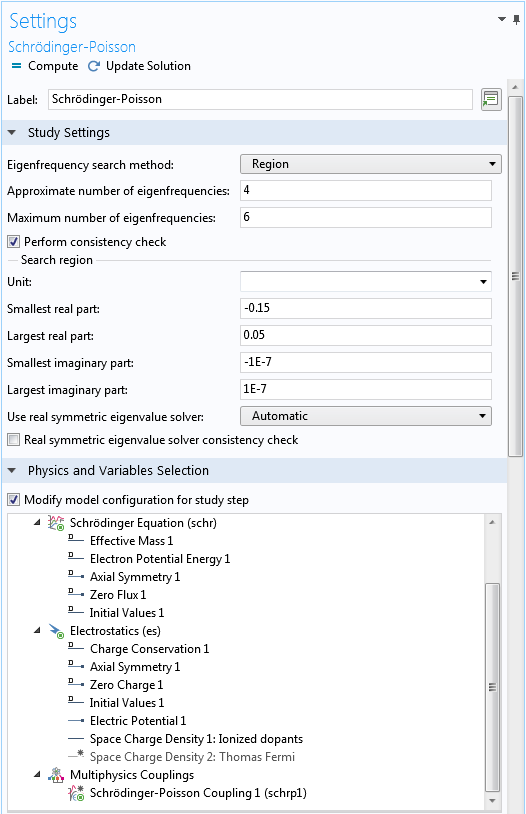
Upper part of the Settings window for the Schrödinger-Poisson study step.

As we have pointed out earlier, the second Space Charge Density domain condition is only used for the Thomas-Fermi approximation solution in Study 1. It is thus disabled under the Physics and Variables Selection section, as shown in the screenshot above.

Under the Iterations section, the default option for the Termination method drop-down menu is Minimization of global variable, which automatically updates a result table that displays the history of the global error variable after each iteration during the solution process. The built-in global error variable schrp1.global_err computes the maximum difference between the electric potential fields from the two most recent iterations, in the unit of V, as already configured in the Schrödinger-Poisson Coupling multiphysics node. (Note that the prefix schrp1 should match the Name input field of the Schrödinger-Poisson Coupling node.) Setting the tolerance to 1E-6 thus means that the iteration ends after the max difference is less than 1 uV. See the screenshot below for these settings:

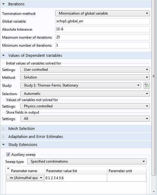
Lower part of the Settings window for the Schrödinger-Poisson study step.

Under the Values of Dependent Variables section, we select the Thomas-Fermi approximate solution from Study 1 as the initial condition for this study. We then use the Auxiliary sweep functionality to solve for a list of nonnegative azimuthal quantum numbers m. The negative ones are taken into account using the formula 1+(m>0) for the degeneracy factor, g_i, as discussed earlier. The dedicated solver sequence automatically performs the statistically weighted sum of the probability densities for all of the eigenstates.

Examining the Self-Consistent Results

The solver converges in eight iterations thanks to the good initial condition provided by the Thomas-Fermi approximation and the good forward estimate of the space charge density given by Eq. 9. The plot of the electron density, potential energy, and partial orbital contributions agree well with the figure published in the reference paper.

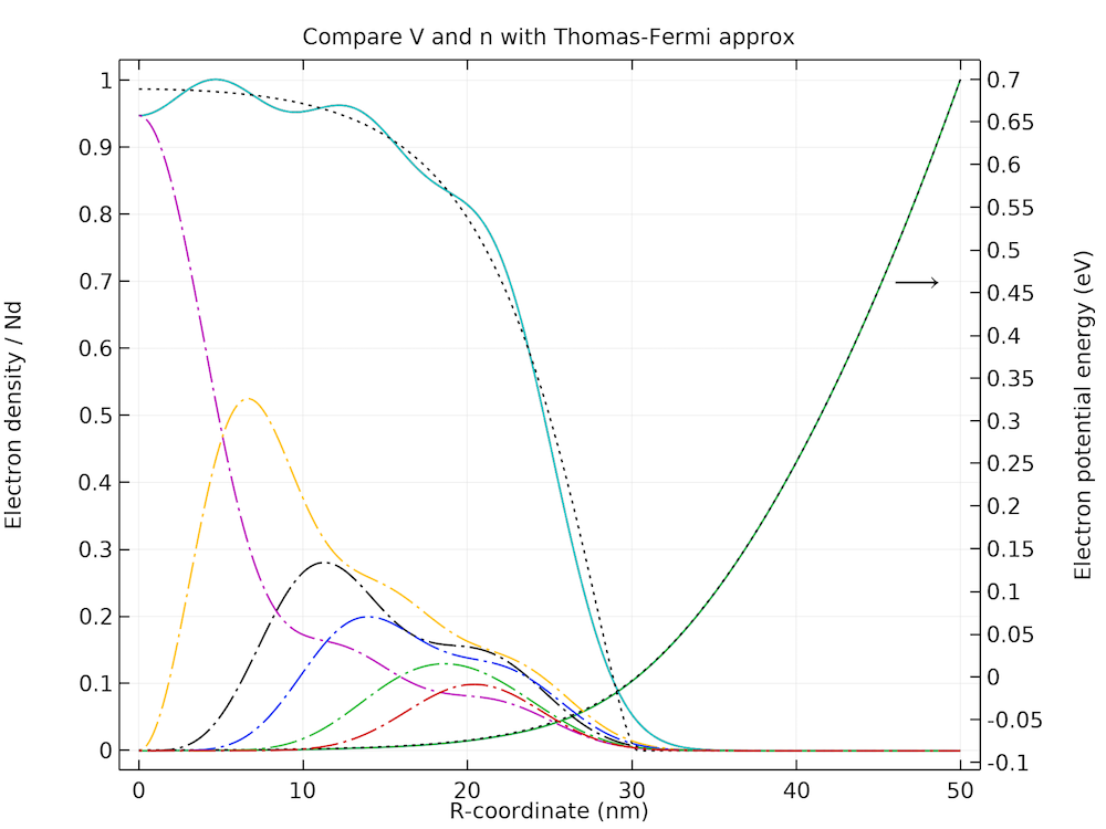
Comparison of the electron density, potential energy, and partial orbital contributions with the figure published in the reference paper.

The plot below shows the Friedel-type spatial oscillations present in both the electron density and the potential energy profiles.

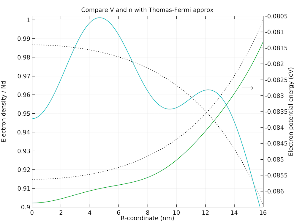
Zoomed-in plot of the Friedel-type spatial oscillations in the electron density and potential energy profiles.

Next Step

In this blog post, we have demonstrated that the Schrödinger-Poisson Equation interface and the Schrödinger-Poisson study type make it simple to set up and solve a Schrödinger-Poisson system, using the Self-Consistent Schrödinger-Poisson Results for a GaAs Nanowire benchmark model as an example. To try this model yourself, click the button below to go to the Application Gallery, where you can download the documentation and the MPH-file for this tutorial.

We hope you find these new features useful and we would love to hear how you apply them to your research.

Reference

1. J.H. Luscombe, A.M. Bouchard, and M. Luban, “Electron confinement in quantum nanostructures: Self-consistent Poisson-Schrödinger theory,” Phys. Rev. B, vol. 46, no. 16, p. 10262, 1992.