The Effects of Varying Solvent Compositions on Lithium-Ion Battery Aging

As lithium-ion batteries age, parasitic reactions can affect the ratio of solvents in the electrolytes. In this blog post, we explore how the consumption of one solvent can impact battery performance over time.

Two Modeling Scales

The liquid electrolyte in lithium-ion batteries typically comprises a lithium salt, such as LiPF6, dissolved in one or more hydrocarbon-based solvents, along with additional additives. In electrolytes that contain multiple solvents, the transport properties within the separator and electrodes may depend not only on the salt concentration but also on the ratio of the different solvents.

As the battery ages, parasitic reactions, such as the formation of a solid electrolyte interface, can selectively consume one of the solvents, altering this ratio over time. Such changes, in turn, can affect how the electrolyte transport properties depend on the local salt concentration within the cell throughout the battery’s lifespan.

To discover how the consumption of one solvent impacts battery performance, we take the approach of using two different modeling scales. Initially, we use molecular dynamics (MD) simulations available in Compular Lab, a web application from Compular, to estimate the transport properties in the electrolyte. The results from Compular Lab are utilized in the Lithium-Ion Battery user interface in the COMSOL Multiphysics^® software. This interface employs a cell-scale model, an extended version of the Doyle–Fuller–Newman lithium-ion battery model, to enhance our understanding. Specifically, we have augmented the original model to include the buildup of a solid electrolyte interface in the negative electrode, which consumes a solvent in the electrolyte solution. The buildup of the solid electrolyte interface is a well-established aging mechanism in lithium-ion batteries.

The Transport Properties

The cell-scale model defines the balances of current, charge, and material (specifically the salt) within the separator electrolyte and the pore electrolyte of the porous electrodes (both positive and negative). It also defines the electrochemical charge transfer reactions occurring within these porous electrodes and the current balance in their electron-conducting structures.

The equations for the balance of current and material in the separator and pore electrolytes (Ref. 1) incorporate transport properties that depend on the solvents in the electrolyte solution. These properties are determined by four model parameters:

• Conductivity, \[{\sigma _l}\]
• Salt diffusivity, \[{D_l}\]
• Transference number, \[{t_ + }\]
• Thermodynamic factor, \[\left( {1 + \frac{{\partial f}}{{\partial {c_l}}}} \right)\] where \[f\] denotes the activity coefficient and \[{c_l}\] the salt concentration

The following equation illustrates the expression for the electrolyte current density vector (\[{{\mathbf{i}}_l}\]), which is utilized in the current balance for the electrolyte. It demonstrates how the conductivity, transference number, and thermodynamic factor parameters influence the migration and diffusion of ions:

1

The equation below accounts for the flux (\[{{\mathbf{J}}_l}\]) of the salt and is integrated into the corresponding material balance. Here, salt diffusivity and transference number affect how diffusion and migration contribute to the movement of salt ions:

2

In the above equations, \[{\phi _l}\] represents the ionic potential (a dependent variable), and \[{c_l}\] signifies the dimensionless salt concentration (also a dependent variable). The symbols \[F\] and \[R\] denote Faraday’s constant and the universal gas constants, respectively. \[T\] denotes temperature, which can be a dependent variable; however, it is held constant in this case.

The values of the four model parameters governing the transport properties depend on the solution’s composition. In our model, we explore a solvent mixture of ethylene carbonate (EC) and ethyl methyl carbonate (EMC), with an initial ratio of EC:EMC at 3:7. These model parameters are computed for varying salt and solvent concentrations using molecular dynamics (MD) simulations in Compular Lab.

MD simulations predict electrolyte properties from first principles, fundamentally involving the solution of Newton’s equations for large systems of simulated atoms and molecules. This process generates significant amounts of data on how individual atoms move, which can later be analyzed to extract material properties such as density, viscosity, and, critically for electrolytes, ion transport properties. The interactions between atoms are governed by classical physics, while the strengths of different interactions are derived from quantum chemistry calculations. These calculations allow us to predict atomic and molecular properties based on our understanding of fundamental physics. Therefore, MD simulations can be applied to any formulation, even those involving chemicals that have never been synthesized. Compular Lab enables users to specify the electrolytes they wish to simulate and automates the MD simulations.

In the simulations outlined below, we fit physically motivated semi-empirical polynomial curves to the data generated by the MD simulations from Compular Lab, which vary across different salt concentrations and EC:EMC ratios. Consequently, the four model parameters previously discussed are transformed into functions of the salt concentration and solvent composition. We then enter these functions into the COMSOL model.

Figure 1 below displays the polynomial expressions for the electrolyte conductivity \[{\sigma _l}\] as a function of the salt concentration (\[{c_l}\]) for various EC:EMC ratios, expressed in percentages. Notably, a 30% value corresponds to the initial ratio of 3:7.

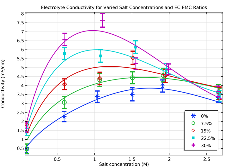Figure 1. Electrolyte conductivity as a function of salt concentration for five different EC:EMC ratios, computed using Compular Lab.

As shown in Figure 1, the conductivity is initially low at low ion concentrations due to an insufficient number of charge carriers for the ionic current. As the salt concentration increases, conductivity reaches a maximum. At higher salt concentrations, the conductivity decreases, a change that can be attributed to reduced ion mobility. This effect is also reflected in the diffusivity curves below.

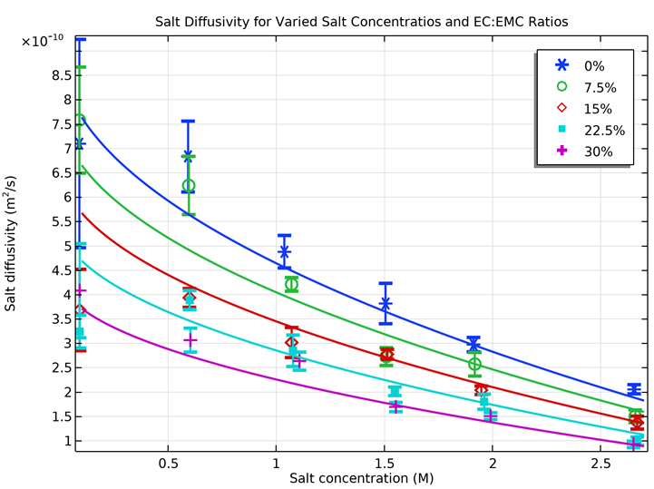Figure 2. Salt diffusivity as a function of salt concentration for five different EC:EMC ratios, computed using Compular Lab.

Figure 2 illustrates the salt diffusivity as a function of salt concentration. The curves indicate that diffusivity decreases with increasing salt concentration, a trend attributable to reduced ion mobility due to stronger “friction” between salt ions. Additionally, the plot reveals that diffusivity declines as the proportion of EC increases. Since EC has a higher viscosity than EMC, this suggests greater solvent–solvent interaction forces, which also contribute to reduced mobility and increased “friction” for ions transported through this solvent.

Counterintuitively, conductivity increases with EC content across most of the salt range, see Figure 1, while diffusivity is lower at higher EC content throughout the entire range. This phenomenon stems from the stronger solvating ability of EC, leading to fewer ion pairs and aggregates, and illustrates the complex relationship between conductivity and diffusivity in concentrated binary electrolytes.

The transference number for the positive ion, which indicates the proportion of the ionic current carried by the positive ions, does not exhibit a definite trend with varying salt concentrations, nor does it reveal any distinct patterns for different solvent compositions. In this study, we computed an average transference number, \[{t_ + } = 0.31\], which was applied consistently across all salt concentrations and EC:EMC ratios.

Figure 3 below illustrates that the thermodynamic factor appears to be independent of the solvent ratio. In this figure, we observe that the activity coefficient, \[f\], varies linearly with the salt concentration. The relationship expressed as \[\frac{{\partial lnf}}{{\partial ln{c_l}}} = 1.35{c_l}\] is applied, resulting in the solid line representing the thermodynamic factor in the plot for all EC:EMC ratios.

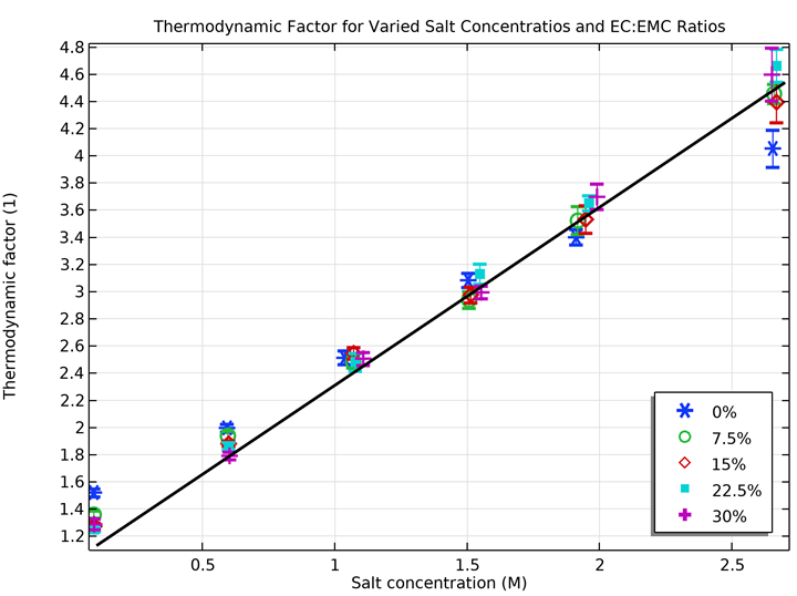Figure 3. The thermodynamic factor as a function of salt concentration, appearing to be independent of the EC:EMC ratios, as computed using Compular Lab.

The Solid Electrolyte Interface

The formation of a solid electrolyte interface (SEI) at the negative electrode is a well-established aging mechanism in lithium-ion batteries. In our model, we assume that the SEI formation reaction consumes EC according to the following electrochemical reaction:

3

The kinetics of this reaction are described by combining the Tafel expression with the limiting current associated with the transport of EC through the SEI (Ref. 2):

4

In the equation above, \[{i_{loc,SEI}}\] represents the local current density for SEI formation, \[{{i_{\lim }}}\] is the limiting current density due to the depletion of EC, \[{{c_{l,ref}}}\] is the salt concentration at the reference state, and \[{{i_{0,ref}}}\] is the exchange current density at the same reference state. The overpotential is denoted by \[\eta \], and \[A\] represents the Tafel slope.

The limiting current density can be estimated from the SEI thickness using the following equation:

5

Here, \[{x_{EC}}\] denotes the mole fraction of EC, \[{i_{lim,0}}\] is the limiting current density at an SEI thickness \[{{s_{SEI,0}}}\], and \[{{s_{SEI}}}\] denotes the current SEI thickness.

To track the growth of the SEI, we formulated a material balance based on Faraday’s law and the kinetics of the electrochemical reaction described above. Since the SEI remains at the location where it forms (i.e., there is no SEI flux), its material balance is represented by a distributed ordinary differential equation, applicable at every point (each x, y, and z coordinate) within the electrode:

6

Here, \[{{c_{SEI}}}\] denotes the concentration of SEI, and \[{A_v}\] represents the specific surface area.

The thickness of the SEI is then calculated as:

7

where \[{V_m}\] denotes the molar volume of the SEI.

The total amount of EC, \[{m_{EC}}\], at any given time is obtained by integrating the SEI concentration throughout the electrode:

8

The mole fraction of EC in the solvent is thus given by:

9

This expression is used in the calculation of the limiting current density described previously.

Porosity and Effective Transport Properties

As the battery ages, the formation of the SEI layer decreases the porosity available for the pore electrolyte, consequently altering the effective transport properties. The electrolyte volume fraction, \[{\varepsilon _l}\], at any given time can be calculated using the following equation:

10

The effective diffusivity and conductivity in the pore electrolyte are then computed using the Bruggeman relation:

11

The Implementation in COMSOL Multiphysics^®

The equations described above are predefined in the Lithium-Ion Battery interface within the Battery Design Module, an add-on product to COMSOL Multiphysics^®, minimizing the manual adjustments required in the user interface (UI). To incorporate a depositing species, we specify a variable for the SEI concentration along with its density and molar mass. Additionally, we add a porous electrode reaction to the negative porous electrode feature. Within this reaction feature, we define the stoichiometry of the electrochemical reaction, select the Tafel equation, and enter a limiting current density. Figure 4 below illustrates how this configuration appears in the UI.

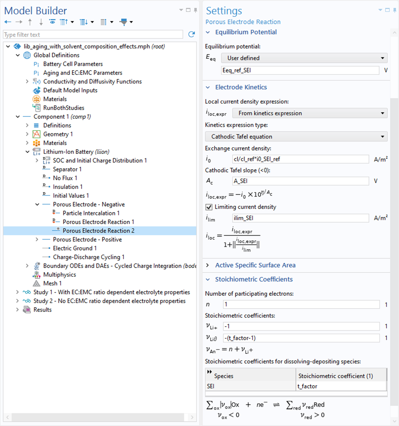Figure 4. Screenshot of the COMSOL Multiphysics UI with the Lithium-Ion interface and with the SEI reaction defined in a Porous Electrode feature.

The Results With and Without Solvent-Dependent Properties

The state of health (SOH) of the battery at a discharge rate of 1C (full battery discharge in 1 hour at constant current) clearly demonstrates the impact of solvent-dependent transport properties. Figure 5 compares the SOH computed from cycles of 1C discharge for two scenarios: one that accounts for solvent-dependent transport properties and another where these properties remain constant. What may be of practical importance in Figure 5 is that when the changes in transport properties are taken into account, the model predicts approximately 200 more cycles to reach 0.9 SOH compared to the case where these changes are not considered.

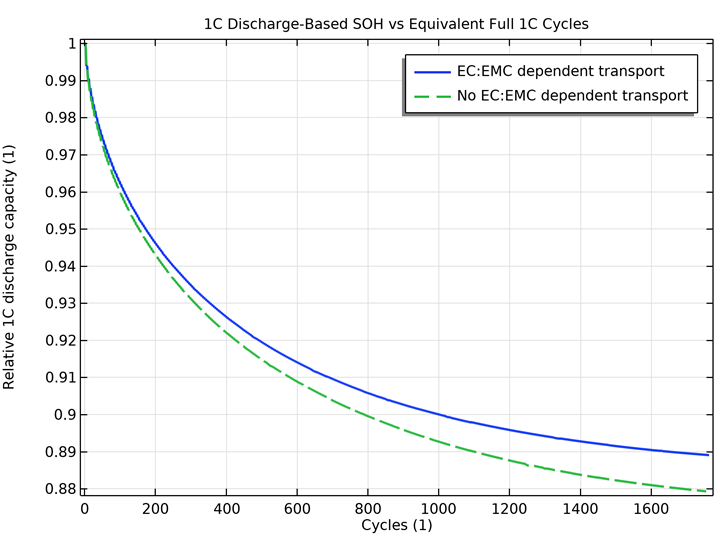Figure 5. Relative discharge capacity at 1C for the solvent-dependent and solver-independent transport properties.

The EC:EMC ratio corresponding to the simulations in Figure 5 is shown in Figure 6. Here, it is evident that both scenarios yield identical results. The EC:EMC ratio decreases from 30% at the initial state to below 2% after 1400 cycles.

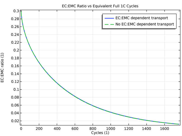Figure 6. EC:EMC ratio as a function of the number of cycles at 1C.

Due to the consumption of solvent, the salt concentration increases with the number of cycles. Figure 7 depicts the salt concentration in the cell as a function of the number of cycles. This, of course, impacts the transport parameters; however, the increase in salt concentration occurs identically in both cases.

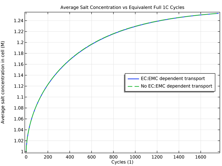Figure 7. Salt concentration in the cell as a function of cycles at 1C for the two cases in Figure 5.

An interesting issue is the extent to which the performance of the cell changes in two scenarios: with and without the effect of solvent composition on transport properties. Figure 8 illustrates the discharge curves for the cell at 100% SOH compared to 90% SOH for both cases.

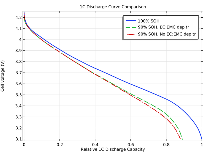Figure 8. Discharge curves for 100% and 90% SOH for the two cases in Figure 5.

Figure 8 demonstrates that the model, which accounts for changes in transport properties with varying EC:EMC ratios, predicts a slightly higher capacity at 1C with an SOH of 90%. Figure 9 presents the total polarization for both cases, indicating that the polarization at 90% SOH is lower for the case that accounts for the solvent properties, beginning at a state of discharge (SOD) of 0.4 and reaching a maximum difference just above 0.8 SOD.

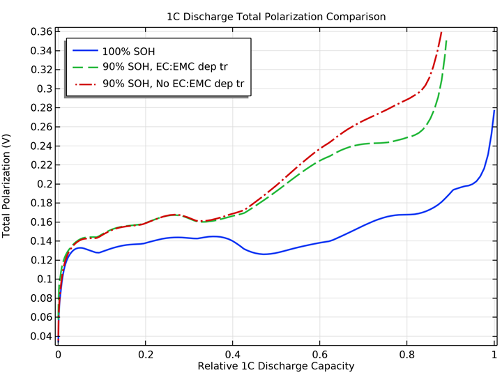Figure 9. Polarization for 100% and 90% SOH for the two cases in Figure 5.

The enhanced performance observed when transport properties are considered is modest yet significant — approximately 40 mV at 0.8 SOD. This improvement can be attributed to higher diffusivity at low EC content. This is further illustrated in Figure 10, which shows the salt concentration at the end of discharge (approximately 0.9 SOD) for both scenarios at 90% SOH. The plot clearly demonstrates that the model, which accounts for varying transport properties in the solvent, leads to a more uniform salt concentration. This, in turn, enhances conductivity and reduces concentration overpotential.

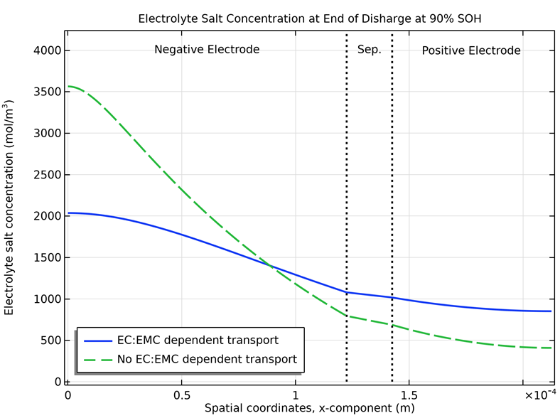Figure 10. Salt concentration at the end of discharge (0.9 SOD) at 90% SOH for the two cases in Figure 5 above.

Integrating Molecular Dynamics and Cell Models to Enhance Prediction Accuracy

We have used two models to simulate aging effects in lithium-ion batteries: one that accounts for varying transport properties as the solvent composition changes during aging (EC:EMC ratio), and a second that does not consider changes in transport properties. We calculated the dependency of transport properties on both the solvent composition and salt concentration using Compular Lab.

The simulation results reveal a modest yet significant impact of the solvent composition on transport properties, resulting in a polarization difference of about 40 mV at 0.8 SOD and 90% SOH. What may be more important is that the case where changes in properties are taken into account predicts 200 more cycles before reaching 90% SOH.

The models presented above demonstrate how such simulation studies can be conducted in COMSOL Multiphysics^® and Compular Lab. However, this is not a full-fledged scientific study. It includes all the components of such a study but is intended to illustrate the principles and the use of the two software platforms.

Next Steps

• Want to try out the model discussed above? Download the related MPH file in the Application Gallery:
  • Lithium-Ion Battery Aging with Varying Solvent Composition Effects
• Interested in learning more about how to generate parameters using Compular Lab? Check out this blog post on Compular’s website:
  • How can we model the effect of solvent breakdown on the performance of your batteries?

References

1. Doyle, J. Newman, A.S. Gozdz, C.N. Schmutz, and J.M. Tarascon, “Comparison of Modeling Predictions with Experimental Data from Plastic Lithium Ion Cells,” J. Electrochem. Soc., vol. 143, no. 6, pp. 1890–1903, 1996.
2. Ekström and G. Lindbergh “A model for predicting capacity fade due to SEI formation in a commercial Graphite/LiFePO4 cell”, J. Electrochem. Soc., vol. 162, pp. A1003–A1007, 2015.