Viscosity Ramping Improves the Convergence of CFD Models

Are you solving turbulent flow problems in your CFD analyses? Then you may be familiar with the large computation time that can result from difficulties in finding the numerical solution. Such difficulties are caused by nonlinearities that arise in the turbulence model equations. Viscosity ramping can help decrease the computation time by solving for higher viscosities and using the solutions as initial conditions for the problem at lower viscosities. We’ll show you how to implement this technique in COMSOL Multiphysics.

Why Does Viscosity Ramping Improve CFD Convergence?

Before starting any fluid flow modeling, you’ll always want to check the Reynolds number, which is defined as:

where \rho denotes the density and \mu is the dynamic viscosity of the fluid. U is a characteristic velocity and d is a characteristic length of the modeled system.

The Reynolds number is the ratio of the inertial forces to the viscous forces in the flow. Calculating the Reynolds number helps to determine which type of analysis — laminar or turbulent — we should perform in COMSOL Multiphysics. For example, in a microfluidic channel where both the characteristic velocity and length are relatively small, the Reynolds number is low and the flow is laminar. In contrast, for a high velocity flow around a car, the Reynolds number is high and the flow is turbulent. You can learn more about characterizing the flow in this earlier blog post.

When solving fluid flow problems using CFD, it is oftentimes more challenging to find a numerical solution to a turbulent flow problem than to a laminar one. To understand why, let’s consider the equations that are solved. For turbulent flow, COMSOL Multiphysics solves the Reynolds-averaged Navier-Stokes (RANS) formulation of the Navier-Stokes equations. The RANS equations introduce a new variable, turbulent viscosity, in order to characterize the turbulence levels in the flow. The turbulent viscosity is calculated using additional equations defined by the turbulence model applied in the simulation.

For instance, the k-epsilon turbulence model uses turbulent kinetic energy (k) and turbulent dissipation (epsilon) to calculate the turbulent viscosity. The turbulence model equations take a similar form to the Navier-Stokes equations, containing both linear and nonlinear terms. The nonlinearities that arise in the turbulence equations explain why achieving convergence is more challenging for high Reynolds number simulations. To learn more about which type of turbulence model to choose, take a look at this blog post.

So, for high Reynolds number simulations, we have to use turbulence models and the equations solved by COMSOL Multiphysics become highly nonlinear. Starting with a good initial condition can help nonlinear problems converge, as described here. Fluid viscosity controls how nonlinear the equations are. By first solving our model with a higher viscosity, we can solve a weakly nonlinear problem that is more likely to converge. Then, we can use the higher viscosity solution as a good initial condition to the lower viscosity problem that we actually want to solve in order to improve convergence. This technique is called viscosity ramping.

With viscosity ramping, we solve a series of models starting with a higher fluid viscosity and decreasing the viscosity until it returns to its desired value. The solution from the more viscous problem is used as the initial condition for the next less viscous problem. We first solve our model with a higher viscosity, thus a lower Reynolds number. This lets us start by solving a weakly nonlinear model that converges more easily. By decreasing the viscosity (and thus increasing the Reynolds number) back to its original value, we shift from a weakly to strongly nonlinear problem, and at the end of the procedure, we have the answer to our original model. Let’s now look at how to do this in COMSOL Multiphysics.

Implementing Viscosity Ramping in COMSOL Multiphysics

Let’s suppose that you already have a CFD model set up in COMSOL Multiphysics and that you want to improve the convergence. Viscosity ramping is a technique that involves three steps:

• Creating a ramping parameter
• Multiplying viscosity by the ramping parameter
• Defining an auxiliary sweep of the ramping parameter in the study

To begin, we define a new parameter that will be multiplied by the viscosity. The value that we set for “visc_ramp” in Parameters is not important, as we will later define an auxiliary sweep that overrides the current value.

Defining the parameter.

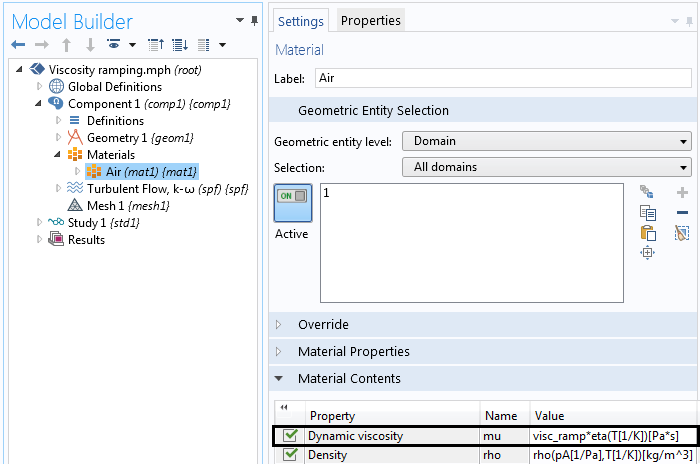
Navigating to the Materials node, we can then multiply the fluid viscosity by “visc_ramp”. For instance, if “visc_ramp” has a value of 100, we would be solving our flow problem with a fluid that is 100 times more viscous than before. Ultimately, when our “visc_ramp” value reaches 1, we return to the actual viscosity of the material.

Multiplying the viscosity by “visc_ramp”.

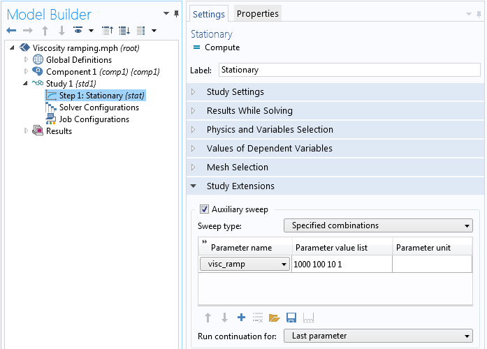
In the Stationary study step, we create an auxiliary sweep of “visc_ramp” for values of 1000, 100, 10, and 1. The auxiliary sweep will find a solution for the first value of “visc_ramp” (1000) and use this solution as the initial condition for solving the next value of “visc_ramp” (100). The sweep continues in such a way until “visc_ramp” reaches a value of 1, which means that we are solving for the actual fluid viscosity.

The Stationary study step.

While computing the study, the Progress tab shows the value of “visc_ramp” that is being solved for at the time. Finally, our solution converges and we can view the results.

The Progress tab for the solution with “visc_ramp” set to 100.

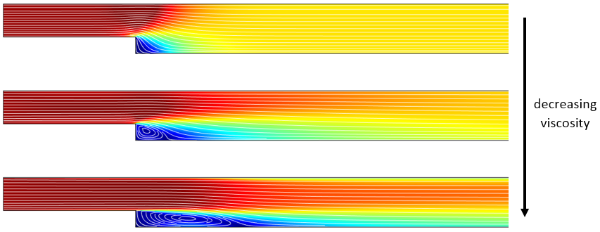
This viscosity ramping procedure is illustrated below. The image shows the streamlines and velocity for turbulent flow over a backward facing step and is based upon the Application Gallery example.

The velocity plot with streamlines of a turbulent backstep for three different viscosities.

Choosing Ramping Parameters for the Sweep

In many situations, starting with a ramping parameter of 100 or 10 is sufficient to assist with convergence. But in cases where convergence is more challenging, it is recommended to use a higher starting value for the viscous ramping parameter and then ramp it down by an order of magnitude each time (i.e., 1000, 100, 10, 1).

Here, we started with a highly viscous fluid (1000) and defined intermediate values of “visc_ramp” (100 and 10) to help the solver transition to the actual fluid viscosity (1). If the solver ever fails to find a solution for the next lower viscosity, then it will try an intermediate value between the last converged value and the next user-specified value — a process known as backtracking.

To demonstrate backtracking, let’s run the auxiliary sweep with 1000 and 1 as the values for “visc_ramp”. After solving for a viscous ramping parameter of 1000, the software will try to solve with a ramping parameter of 1. Once the solver notices that convergence is not being reached, it will backtrack and try an intermediate value of the ramping parameter (in this case, 501). After the solution converges with the backtracking parameter value of 501, it will then attempt to solve with a viscous ramping parameter of 1 again, and this time, it will do so with success!

The Progress tab for the solution with “visc_ramp” set to 501.

Backtracking is a valuable built-in technique that the solver uses to improve convergence during an auxiliary sweep. However, the user should still specify intermediate values in the sweep to help the solver transition from the higher to the lower ramping values.

In some situations, the solver will use backtracking and stop converging at a value larger than 1. This is typically a sign that the mesh is too coarse to resolve the flow field. In such a case, you should first refine the mesh. Further, keep in mind that you will always want to do a mesh refinement study as part of your model verification procedure.

The Power of Viscosity Ramping and Nonlinearity Ramping

We have shown you how to use viscosity ramping in COMSOL Multiphysics to help a CFD model converge. To do so, we set up a continuation study so that we start with a weakly nonlinear problem and then progressively increase the nonlinearity until the original problem is solved. This viscosity ramping technique can be quite helpful in solving CFD problems at large Reynolds numbers when turbulence models are required.

The technique of nonlinearity ramping can be applied in many different ways. For instance, instead of viscosity ramping, we can ramp the gravitational force in natural convection problems or the flow behavior index “n” in non-Newtonian fluid flows. It can also be used more generally in any nonlinear multiphysics problem, as highlighted here.

In a process similar to nonlinearity ramping, we can instead ramp the load in a system to improve convergence. Load ramping in fluid flow usually means ramping the inlet velocity and is another technique that you will want to keep in mind.

Want to learn more about these techniques and applying them to your own COMSOL Multiphysics simulations? Please contact us today.