
Exploring the Partial Fraction Fit Functionality in COMSOL Multiphysics®

Today, guest blogger René Christensen of Acculution ApS discusses the Partial Fraction Fit feature, introduced in version 6.2 of the COMSOL Multiphysics® software.
In version 6.2 of the COMSOL Multiphysics® software, there is a new Partial Fraction Fit function. This feature analyzes a complex-valued function of frequency given through its real and imaginary parts. It results in a sum of several fractions that fit the function and describe the system in a very compact way over the frequency range in question. The fractions are known as partial fractions that together make up a numerical transfer function, which is relevant for gaining insight into the inner workings of the underlying system and also makes for an easy transformation to the time domain. The real and imaginary parts of the input values will typically come from a priori simulations, but they can also be imported values from other software or even other measurements.
Table of Contents
- Time-to-Frequency Transformation
- Transfer Functions
- Partial Fraction Decomposition
- Partial Fraction Fitting
- Real Poles
- Complex Poles
- Repeating Poles
- Unstable Poles
- Nonrational Transfer Function: Time Delay
- Nonrational Transfer Function: Microacoustics
- Conjugate Symmetry, Negative Frequencies
- Concluding Thoughts
Time-to-Frequency Transformation
As the functionality involves frequency-domain analysis, it is informative to briefly look at some aspects of working in the frequency domain and how to get there for signals and systems.
While signals in general vary over time, it is often easier to analyze them in the frequency domain. Similarly, systems are most often analyzed by converting aspects of their time-domain characteristics to the frequency domain. Conversion between the time and frequency domains is typically done either via the Fourier or Laplace transform and their respective inverse transforms. While there is a great overlap between the two, here we will focus on the Laplace transform, as this is traditionally the one used for systems analysis. The Laplace transform is given as the unilateral integral:
where s is a complex frequency defined via the angular frequency, \omega, and damping, \sigma, as
This unilaterality makes this integral suitable for systems, as they can then have a particular time at which they are “turned on”, and transient behavior can be investigated. Also, the Laplace transform will serve as the primary transform for establishing the transfer functions discussed later. A few important time–frequency pairs are listed in the table below:
| f(t) | F(s) |
|---|---|
| kf^{(n)}(t) | s k F(s) + k f(0) |
| k \int^{t}_0 f(\tau) d\tau | k\frac{F(s)}{s} |
| t^n e^{-\sigma_0 t} | \frac{n!}{(s+\sigma_0)^{n+1}} |
| ke^{-\sigma_0t}\cos(\omega_0t) | k \frac{s + \sigma_0}{(s + \sigma_0)^2 + \omega^2_0} |
| ke^{-\sigma_0t}\sin(\omega_0t) | k \frac{\omega_0}{(s+\sigma_0)^2 + \omega^2_0} |
Transfer Functions
Many systems can be described via linear differential equations with constant and real coefficients, forming so-called real and linear time-invariant (LTI) systems. An example could be a mass–spring–damper system with a velocity (output), v, for an external force (input), f_\textrm{ext}, as:
where m is mass, r is resistance, and k is stiffness. Here, we write in terms of velocity instead of displacement or acceleration since force and velocity are power conjugate variables, just as voltage and current in electrical systems are.
The Laplace transform is then performed under the steady-state assumptions that oscillatory, possibly damped, complex exponential phasor inputs and outputs are of the form F(s) = (F_0e^{\phi_F(s)})e^{st} and V(s) = (V_0e^{\phi_V(s)})e^{st}, respectively, where F_0 and V_0 are real numbers. These assumptions lead to the frequency-domain description of the system:
We ignore initial conditions here, but they can also be included in the above equation. Since we are often interested in what the resulting output, Y(s), for some input, X(s), is, we can use a general transfer function:
For the present system, this yields the transfer function:
It is very common in engineering dynamics that the transfer function associated with an LTI system will be a rational function, which is a fraction of two univariate polynomials involving only the variable s as:
This can alternatively be written in a form of factored zeros and poles as:
where
One notable aspect of rational transfer functions is their order, which is the highest degree of s in the denominator here, given directly by the exponent n. Another aspect is their properness. There are three categories to consider. One is called proper, for which the order of the denominator is higher than or equal to the order of the numerator; that is, n \geq m. Another is a subset called strictly proper, where the number of poles is (strictly) higher than the number of zeros; that is, n > m. Finally, the third category is improper, for which n < m. In the last case, you should consider potential stability and causality issues, but the properness is also affected by whether the analysis is done for a particular transfer function or for its inverse.
For a mass–spring–damper system, the transfer function falls in the category of a bandpass filter, which makes sense, since at a particular frequency there will be a resonance in velocity for the applied force. With the standard form for a bandpass function being
we can find the characteristic angular frequency:
and
The order of the mass–spring–damper system is two. This also means that there are two associated roots of the denominator polynomial: the poles. For the real systems considered here, there are three possibilities for the two poles: 1) two distinct real poles, 2) two real, overlapping (repeating) poles, or 3) two complex conjugate poles. The roots of the numerator are called zeros, and the zeros and poles will fully describe the linear time-invariant real-coefficient systems of interest, provided that the region of convergence (ROC) is known. Here, we assume causal systems, and so the ROC will be known via that information. This will lead to stable systems not having poles in the right-hand plane of the complex s-plane. It will also ensure that a Fourier transform exists, which is needed to justify finding a frequency response from the transfer function. With the systems being real, there is conjugate symmetry, and so, as mentioned already, complex poles will always come in conjugate pairs.
Partial Fraction Decomposition
When learning about transfer functions and (inverse) Fourier/Laplace transform, one might come upon the topic of partial fraction decomposition (PFD). Here, the incentive is typically to make it easier to find inverse Laplace transforms via tables. Higher-order transfer functions can be broken down into simpler fractions, and their inverse transforms will add up to the total inverse since linearity holds for the systems in question. It may also be relevant when solving integrals containing integrands that are rational functions. And finally, in control theory it can be of interest to break down a higher-order transfer function into several lower-order fractions.
We will now illustrate the procedure for decomposing a transfer function into its partial fractions, where the poles could be written in a factorized form. The transfer function is of order 5, with a dual repeating pole of -5 and a triple ditto of 0, and so we will need five partial fractions:
Multiplying with the general denominator, we get:
Comparing the different orders of the left- and right-hand sides, the unknowns can be found as A=0.52, B = -1.6, C=4, D=-0.52, and E=-1.
Using tables for the inverse Laplace transform, one can thus find the impulse response of the associated system as:
Having to do this inverse transform directly from the original transfer function would require the use of mathematical software, but with partial fraction decomposition it is doable analytically by hand, at least when the zeros and poles are known numerically. Note that for improper transfer functions, one may need to do polynomial long division to split the original transfer function into an asymptotic value and subsequent fractions.
The time-frequency relationship is taken advantage of with the new option of having frequency-dependent impedance in time-dependent acoustics, using the Partial Fraction Fit (PFF) function.
Partial Fraction Fitting
While it is typically not possible to find an analytical transfer function for a simulated multiphysics problem, one can still find a ratio between an output and an input as tabulated complex values. These values can be the output of a simulation or, alternatively, be imported values from a measurement. Now, if there was a way to establish a transfer function from the tabulated values, one could gain insight into the system that would be difficult to discern directly from the values on their own. Then it would also be possible to perform an analytical inverse Fourier transform to form the impulse response, instead of having to perform, for example, an inverse fast Fourier transform study. Finally, describing the system in terms of zeros and poles instead of a large table of data compactifies the system, while retaining all of its characteristics, at least within the chosen frequency range for tabular values. This is basically what is now possible with the Partial Fraction Fit feature in COMSOL Multiphysics® — establishing a numerical transfer function via complex values as a function of frequency.
In the PFF function node, values are input from tables, holding real and imaginary numbers as well as the frequency. The PFF will then fit those values, resulting in a partial fraction version of the transfer function describing the underlying system. The PFF is based on a “modified adaptive Antoulas–Anderson (AAA) algorithm, AAA2” (found in the COMSOL Multiphysics Reference Manual) with the mathematical form:
The first part is simply the asymptotic value related to the properness of the fitted system, and we see via examples how this comes into play. The first summation is over all real-valued poles that the fitting function finds, with the residues also being real. The second summation is over the complex-valued poles that the fitting procedure finds, with the residues also being complex. It is seen that the complex poles and residues are expected to come in complex conjugate pairs, with one complex pole being a mirrored twin of the other. It will be discussed later how this assumption of conjugate symmetry on the PFF result does not extend to the underlying system input from where the values came, and so there is no restrictions on those systems being real or physically realizable.
It should also be noted that in the above expression, x is frequency, as opposed to the angular frequency \omega used when detailing the transfer function basics. Also, the fractions are all of first order with constants in the numerator, and so for repeating poles, it may take a little work to reformulate into the form shown for the partial fraction decomposition technique, where the numerator may have higher orders in general. Other than that, the PFF essentially returns a numerical transfer function in a partial fraction form, and so fundamental signal processing knowledge comes in handy, including now, as we probe the functionality with different examples.
Real Poles
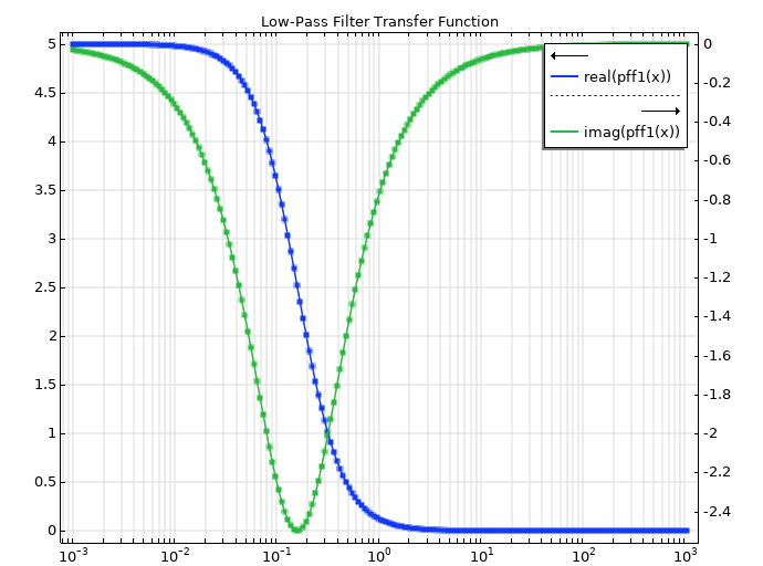
To look at how this functionality can be used to find real poles, we apply the PFF to known simple, analytical transfer functions to get a feel for how it operates and what it returns. First, we test the output of the PFF for a first-order low-pass filter function:
Here, there is one real pole of p = -1, with the real residue being 5, when the factor/coefficient K_\textrm{DC} is absorbed into the numerator. We will now see if the PFF function can find it. Knowing the transfer function, we can calculate the real and imaginary values for its frequency response. Next, we feed the values into the PFF. We can plot the tabular values (square markers) alongside the fitted values (solid line) and see how well the fit has been made. In this case, there is seemingly a perfect match, but it is informative to not only look at the curves, but also investigate the actual outputs.
The PFF results shown are for the fitted residue and pole values:
| Parameter | Value | Value scaled by 2\pi |
|---|---|---|
| Y_\infty | 6.547\cdot 10^{-15}+3.78\cdot 10^{-16}i | N/A |
| R_1 | 0.796 | 5 |
| \xi_1 | -0.159 | -1 |
The asymptotic value is essentially zero, which is what was expected for this type of rational function. The pole is also found correctly, since the x in the PFF is frequency in Hz, and not angular frequency in radians per second, such that the pole in the transfer function is 2\pi higher than the pole found via the PFF. Since this scaling goes through the entire equation, the residue of 0.796 is about 2\pi lower than the expected 5 \cdot 1, and so everything fits together with the proper scaling.
Another real poles case is investigated with the following transfer function:
The poles are directly seen from the transfer function, and we can calculate the partial fractions manually and get:
So, we expect that within a frequency scaling, we will get one residue of 1 for a pole \text{p}=-1, and another residue of -1 for a pole \text{p}=-2. And that is essentially what we get:
| Parameter | Value | Value scaled by 2\pi |
|---|---|---|
| Y_\infty | 7.151 \cdot 10^{-12} – 1.513 \cdot 10^{-11} i | N/A |
| R_1 | -0.159 | -1 |
| \xi_1 | -0.318 | -1.998 |
| R_2 | 0.159 | 1 |
| \xi_2 | -0.159 | -1 |
The asymptotic term is essentially zero, and if we multiply the poles and residues with 2\pi and flip their order, we get the expected values. So, multiple real poles are handled correctly.
Complex Poles
Another example going toward more physical systems is the pressure output from a lumped loudspeaker driver in a baffle. The simple lumped circuit is shown below:
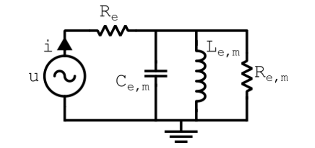
The pressure output will be proportional to a second-order transfer function given as:
with
and
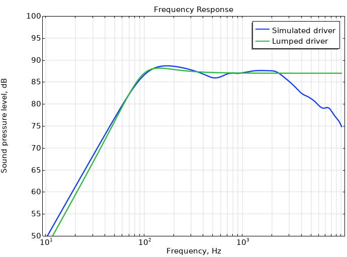
The sound pressure level is shown below, both for the underlying simulated driver serving as inspiration for our lumped model, and the lumped parameters that can be found in the table below.
| Lumped Parameter | Value | Unit |
|---|---|---|
| Bl | 5 | T \cdot m |
| R_e | 6 | \Omega |
| M_m | 13 | g |
| K_m | 5 | N/mm |
| R_m | 4 | N\cdot s/m |
| L_{e,m}= Bl^2/K_m | 5 | mH |
| C_{e,m}= M_m/Bl^2 | 520 | \mu F |
| R_{e,m}= Bl^2 /R_m | 6.25 | \Omega |
| \omega_0 | 620 | 1/s |
| Q_t | 0.98722 | 1 |
With the Q-value in question, we have ensured complex poles at approximately s_{1,2} = -314 \pm 534 i in angular frequency, or x_{1,2} = -50 \pm 85 i in regular frequency. We set K in the transfer function equal to 1, as it simply scales the function, and run the lumped model analysis. The PFF fed with the transfer function values returns the following values:
| Parameter | Value |
|---|---|
| Y_\infty | 1+2.85\cdot 10^{-15} i |
| R_1 | -5.697\cdot 10^{-13} |
| \xi_1 | 99.992 |
| Q_1, Q^\ast_1 | -99.982 \pm 55.744 i |
| \zeta_1, \zeta^\ast_1 | -49.991 \pm 85.108 i |
The asymptotic term is basically equal to one, which is the expected value for this proper, but not strictly proper, transfer function. There is one real pole, alongside two complex poles. The real pole is seen to be unstable, but it has such a low residue that it can simply be deleted. The remaining complex poles have numerical values that fit with the transfer function, and so from here you could, for example, find the transient response using the PFF results. The PFF could also be run on the underlying driver simulation data instead of the approximated lumped model. In such a case, more poles would be found, but the approach would be the same as for the lumped model.
Repeating Poles
Transfer functions can have repeating poles, such that several poles reside in the same place in the s-plane. As covered in the Partial Fraction Decomposition section of this blog post, when doing analytical partial fraction decomposition of such cases, it is common to split the sum into fractions where some denominators have an order higher than one, whereas the PFF only returns first-order fractions. The returned values from the PFF will still be correct, but it was determined that there is high sensitivity to the values found, and so you should not truncate the calculated poles or residues if they are, for example, to be exported and used in some other software.
Unstable Poles
When performing partial fraction fitting, unstable poles may be found. In such cases, you should first look at the residues of these poles and compare them to the residues of the stable poles. The unstable poles with negligible residues can be removed without affecting the overall fitting. If the unstable poles have a significant impact on the fitting accuracy, you should consider what type of underlying system is being investigated. If a system is passive, then it is inherently stable, and so having an understanding of signal processing basics can help in determining issues with simulations or measurements exhibiting unstable behavior in the frequency range of interest. The PFF function provides an option called Flip Poles, which will mirror the unstable poles onto their stable position in the s-plane. This may affect the fitting accuracy, but its effect can immediately be evaluated by replotting the new fit. The unstable poles are often located near the lower frequencies, and so flipping them may only slightly affect the lower frequencies while retaining the higher-frequency behavior.
In general, flipping unstable poles will affect the phase response while retaining the magnitude response, but remember that the causality assumption must be considered for the correct stability interpretation. Also, having most or all poles be unstable may indicate that the data being fitted corresponds to the inverse of a stable function, and thus it can be a good idea to instead evaluate the inverse function.
It should be noted that observations regarding unstable poles and/or repeating poles should be carried out for more transfer functions to get a better grasp of the functionality, so the above analyses should not be seen as exhaustive, but rather introductory only. Also, it can be relevant to investigate formal definitions of passivity of systems (Refs. 1 and 2) without going further into the associated conditions in the present text, other than stating that this passivity check can generally be done by evaluating if all real values in the fitted data are positive.
Nonrational Transfer Function: Time Delay
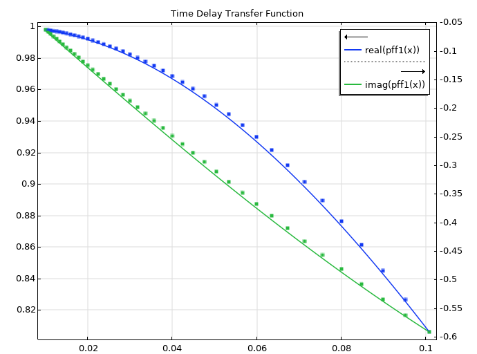
Not all physical phenomena are easily described via rational transfer functions, so we will now look at how well the PFF fits nonrational transfer functions. The first example is a time delay of T seconds, which represents an important transfer function without being in a traditional rational form:
The transfer function is calculated over a particular frequency range with a time delay of one second, and for this frequency range and a particular set tolerance, the PFF returns an asymptotic term of approximately minus one and a single real pole.
| Parameter | Value |
|---|---|
| Y_\infty | -1+3.405 \cdot 10^{-16} i |
| R_1 | 0.6155 |
| \xi_1 | -0.3078 |
The curves are seemingly fitted nicely:
However, we can take it further. Based on the asymptotic value, we know that the transfer function is of the proper kind. We can collect terms and figure out the exact transfer function:
From looking at the numerical values, we can see that the residue value is the opposite to twice the value of the pole. And so, the above expression can be rewritten as
And now we see that what has been achieved is an allpass filter of order one, which makes sense since the magnitude response of a time delay must be flat. But we can take it even further. For an order of one in the numerator and denominator, we can simply find the Padé approximant P_{1,1}(s) — which is equivalent to the Bilinear transformation — for H(s) = e^{-sT}, with the result:
This looks very much like the PFF result. In fact, when converting the above expression to ix format, for T=1 we get:
And with 1/\pi = 0.3183, we can see that the result only has a small percentage difference with what the PFF has given us. For a larger frequency range, more poles would be needed, and it would likely be seen that the poles found represent Bessel polynomials roots (Ref. 4).
Nonrational Transfer Function: Microacoustics
The next nonrational test transfer function is found for a microacoustics case. Consider a rectangular slit with a cross section as shown below (Ref. 5):
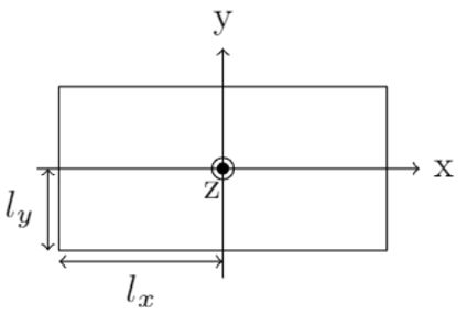
A tube of this cross section will have an associated acoustic series impedance per unit length, Z^\prime, as well as an acoustic shunt admittance per unit length, Y^\prime. These are not directly written in a rational function form, but they can be approximated via active and reactive components at lower frequencies, and it will be interesting to see what can be achieved with the PFF.
We assume that the slit is very thin: l_y \ll l_x. Such a slit will have a series impedance per unit length as follows (Ref. 5):
Here, S = 4l_x l_y is the area of the thin slit; \rho_0 is the density of the air; and x_v = i \omega l^2_y/v, where v = \mu_0 / \rho_0 and \mu_0 is the viscosity of the air. One approach to simplifying this expression is to apply a Taylor expansion to arrive at a lumped model as follows (Ref. 5):
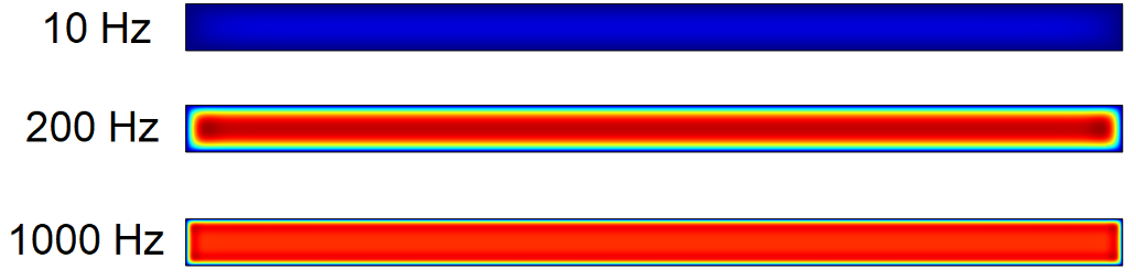
The series impedance at low frequencies can be split into an active and constant resistance part and a reactive and constant mass part. This can be viewed as an improper transfer function, but it will only hold for lower frequencies. So, let’s instead see what the PFF can find. A 2D simulation was set up that could calculate and return the impedance considering both acoustical and microacoustical effects across a particular frequency range, revealing the underlying system characteristics. We must also choose some numerical values for the geometry parameters. Here, l_x is set to 1 cm, and l_y is set to 0.5 mm. The viscous boundary layer is clearly seen to vary as a function of frequency and spans the space of both large and small thickness across the audio range for the chosen geometry dimensions.
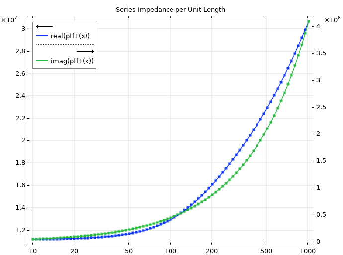
We now feed the calculated series impedance to the PFF functionality. Since there are no explicit zeros or poles to point out in the analytical expression, we have no immediate guess for the outcome of the PFF. The fitting procedure nicely finds suitable parameters for residues and poles to achieve matching curves for the series impedance, and it can be seen how the real part is constant toward lower frequencies (Poiseuille flow), as already seen in the lumped model.
The PFF returns some finite asymptotic value and three real poles:
| Parameter | Value |
|---|---|
| Y_\infty | 9.336 \cdot 10^{10} + 0.135i |
| R_1 | -1.631\cdot 10^{10} |
| R_3 | -1.901 \cdot 10^9 |
| \xi_1 | -237665.182 |
| \xi_2 | -935.471 |
| \xi_3 | -217.677 |
Knowing the number of poles that the PFF finds when fitting in the chosen frequency range, we can now try and make sense of this result. While the series impedance is not described via a rational function but instead a trigonometric function, we can still approximate it via Padé approximants. Since we have a nonzero asymptotic term and three poles in the PFF, the P_{3,3} approximant is the one to look for:
Here, a = \rho_0/S and b = l^2_y/v. Work it all out, and you basically get what the PFF returned.
While the series impedance per unit length was known a priori analytically because of the simplicity of the geometry, it is extra informative to be able to see the fit with an analytical approach for establishing the transfer function. But the actual use case here is, of course, to fit the numerical results for a given simulation without any underlying mathematical expression.
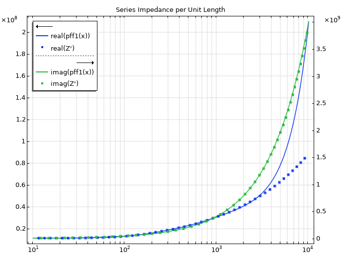
The frequencies chosen here are rather low, and so it is of interest to investigate how well the fit matches at higher frequencies. From looking at the behavior of the exact impedance toward higher frequencies, the underlying transfer function is seen to be improper. Since the PFF functionality by design returns a fitted transfer function of the proper type, we should expect to see a deviation between the exact impedance and the fitted values at higher frequencies outside of the input frequencies, and that is what is illustrated in the figure below. Any fit will take into consideration only the frequency range provided for the PFF, without any guarantee regarding the fit outside of this range. This also ties in with the asymptotic behavior of Padé approximants, but we will not go into those details here. Finally, it should be noted that you can investigate the inverse of any relevant system, which will change the properness for a rational transfer function, but even so, deviations are to be expected outside the frequency range used in the fitting procedure.
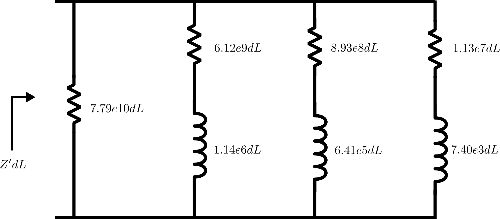
Finally, a circuit can be synthesized from the partial fraction fitting results, as shown below. This will approximate the series impedance for a small slit length, dL, to the same accuracy as the PFF poles and residues in the same frequency range. The details of this synthesis is beyond the scope of this blog post, but it should be mentioned that a shunt admittance should also be established in a similar fashion for a complete description of the slit.
Conjugate Symmetry, Negative Frequencies
As mentioned already, the complex poles in the PFF will present themselves in complex conjugate pairs. However, it is not an explicit constraint that the original system be real, and so it may or may not have an inherent conjugate symmetry associated with it. As the PFF itself has this assumption of conjugate symmetry, one must limit the frequency range for the input values to either positive frequencies, possibly including 0 Hz, or negative frequencies, possibly including 0 Hz. The former is probably much more common than the latter, but both options are available. As there may not be conjugate symmetry in the initial data, the two options may not lead to the same fitted approximant.
Concluding Thoughts
It has been shown here how the new Partial Fraction Fitting feature in COMSOL Multiphysics® behaves for different scenarios, such as strictly proper, proper, and improper rational transfer functions, as well as for nonrational system characteristics such as time delays, microacoustical effects, or coupled multiphysics simulation results. The functionality performs excellently, and it allows for manual fitting thanks to the options for changing frequency range and tolerance as well as for directly changing the values for residues and poles.
It should be noted that for some of the tested transfer functions with real poles (over infinite frequency range), the PFF would sometimes return complex poles in its finite frequency range. However, the imaginary parts were then very small compared to the real part, and it was easy enough to realize how this still made sense numerically. Watch out for such cases, as they can be further simplified by only including the real part. You can also sometimes see very low residues, and so the associated pole might not be of much importance and thus could be removed from the PFF. You can also add or remove poles and residues and see the effect on the fitted curves, which is a very useful feature.
I am very pleased with this functionality in the newest version, and I can imagine a lot of relevant use cases.
Try the Partial Fraction Fit Function
Want to try out the Partial Fraction Fit function for yourself? Check out the Input Impedance of a Tube and Coupler Measurement Setup: Time Domain MOR using Partial Fraction Fit model in the Application Gallery.
References
- B. D. O. Anderson and S. Vongpanitlerd, Network Analysis and Synthesis, New Jersey: Prentice-Hall, Inc., 1973.
- Y. Miki, “Acoustical properties of porous material – Modifications of Delany-Bazley models -”, The Journal of the Acoustical Society Japan, vol. 11, no. 1, pp. 19–24, 1990.
- A. V. Oppenheim and R. W. Schafer, Discrete-Time Signal Processing, New Jersey: Prentice Hall, Inc., 1989.
- J. R. Martinez, “Transfer Functions of Generalized Bessel Polynomials”, IEEE Transactions On Circuits And Systems, vol. CAS-24, no. 6, 1977.
- M. R. Stinson, “The propagation of plane sound waves in narrow and wide circular tubes, and generalization to uniform tubes of arbitrary cross-sectional shape”, J. Acoust. Soc. Am. 89 (2), 1991.


Comments (2)
Avi Sigma
September 26, 2024its difficult!
Acculution ApS
September 27, 2024Any particular part?