Techniques for Creating High-Quality Visualizations of Models
When visualizing results and creating images in COMSOL Multiphysics®, it can be important to create plots that not only display the simulated results but also create a more comprehensive model composition. Creating a more visually impactful model can aid in the demonstration and understanding of your model to colleagues or customers. Here, we will review, demonstrate, and outline some best practice approaches to the different visualization tools available in COMSOL Multiphysics®.
Note: Users who are new to creating plots and visualizations can start by watching the Results section of the Getting Started series.
Datasets
Most plots created underneath the Results node reference a dataset that either contains a solution or links to another dataset with a transformed version of the solution. Most datasets map to a previously created dataset and can build upon one another, referring to the evaluation of the chosen dataset. Solution datasets are an exception and do not map to a previous dataset. They are automatically created when the study of a model is computed. This article will discuss the following commonly used dataset types, as well as their respective 2D and 1D equivalent versions: Cut Planes, Array, Mirror, Revolution, and Sector.
 The Model Builder tree with the Datasets node highlighted, its option menu open, and the More 3D datasets hovered over to show more datasets to choose from.
The Datasets menu and subsequent More 3D Datasets submenu showing some of the available datasets.
The Model Builder tree with the Datasets node highlighted, its option menu open, and the More 3D datasets hovered over to show more datasets to choose from.
The Datasets menu and subsequent More 3D Datasets submenu showing some of the available datasets.
There are various dataset types available that enable you to produce more appealing or complete visualizations. Cut Planes, Cut Lines, and Cut Points datasets can be used to create and analyze cross sections of your model. The Array 1D, 2D, and 3D datasets and Mirror 2D and 3D datasets are effective for duplicating parts of your model geometry. For Array datasets, you can set the displacement, size, and number of cells in 3D space and duplicate the selected geometry accordingly. The Mirror datasets can also be useful when a geometry is sectioned for computational reasons or is part of an axisymmetric problem where it is beneficial to visualize the complete model. The images below depict the results of using the Mirror 3D and Array 3D datasets on the Four-Point Bending Test of an IGBT Module model.
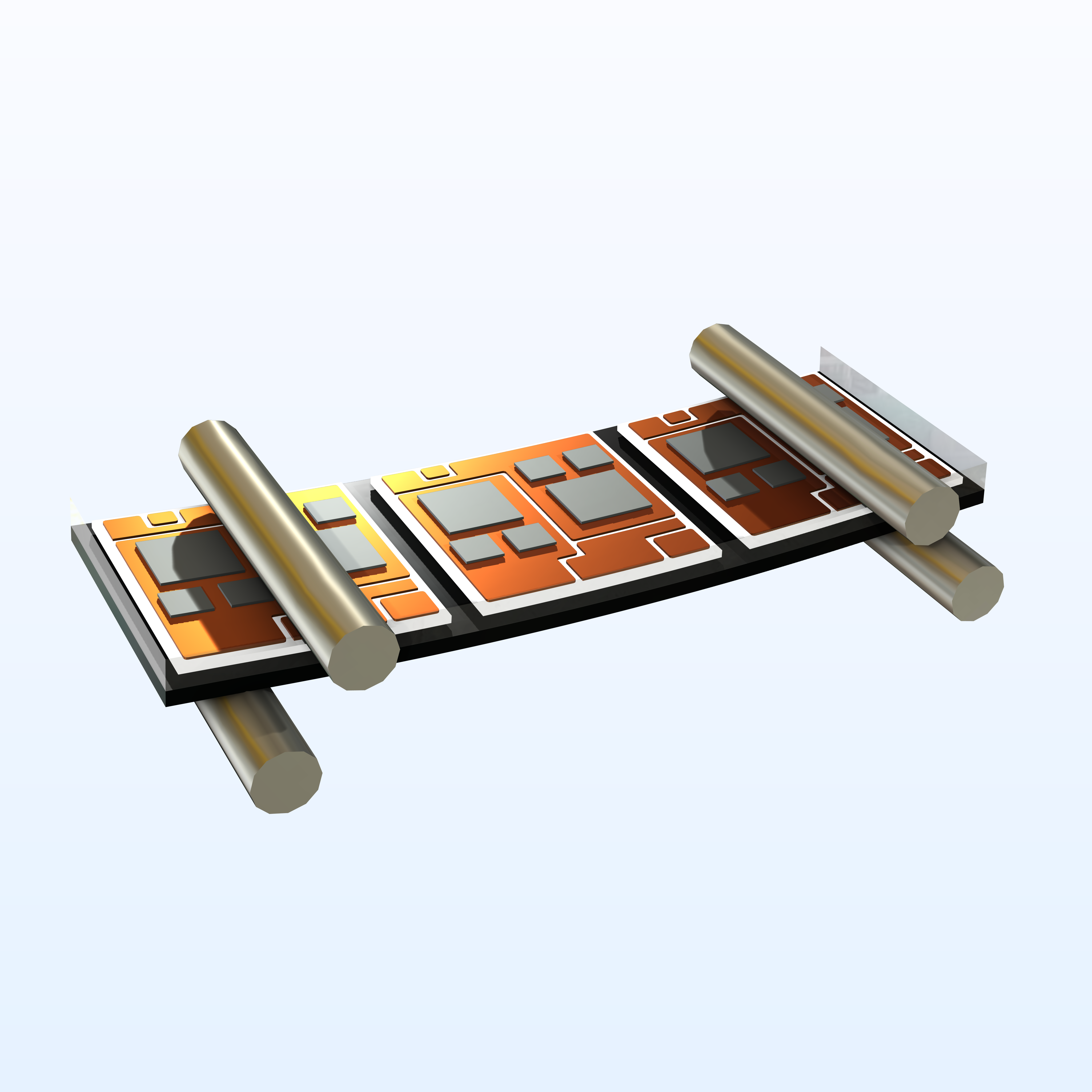 An IGBT module model visualized with its original solution that is equal to a half of its full geometry.
An IGBT module model visualized with the preset Solution dataset. To save computational costs, this model was created and solved using half of its normal geometry.
An IGBT module model visualized with its original solution that is equal to a half of its full geometry.
An IGBT module model visualized with the preset Solution dataset. To save computational costs, this model was created and solved using half of its normal geometry.
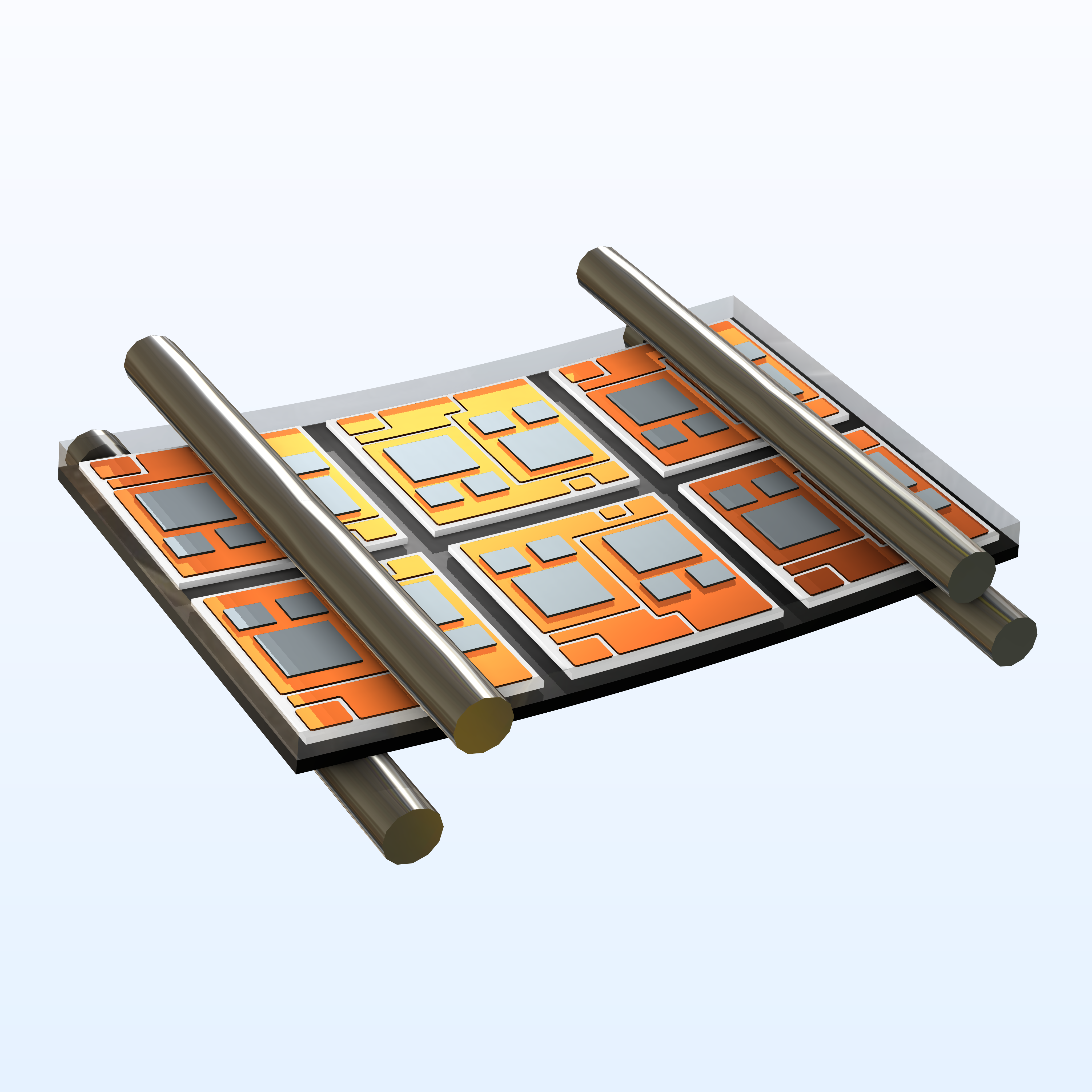 An IGBT module model with its original half geometry mirrored to create the complete geometry.
An IGBT module model visualized using only the Mirror 3D dataset to mirror the entire initial solution to reproduce the actual geometry's appearance.
An IGBT module model with its original half geometry mirrored to create the complete geometry.
An IGBT module model visualized using only the Mirror 3D dataset to mirror the entire initial solution to reproduce the actual geometry's appearance.
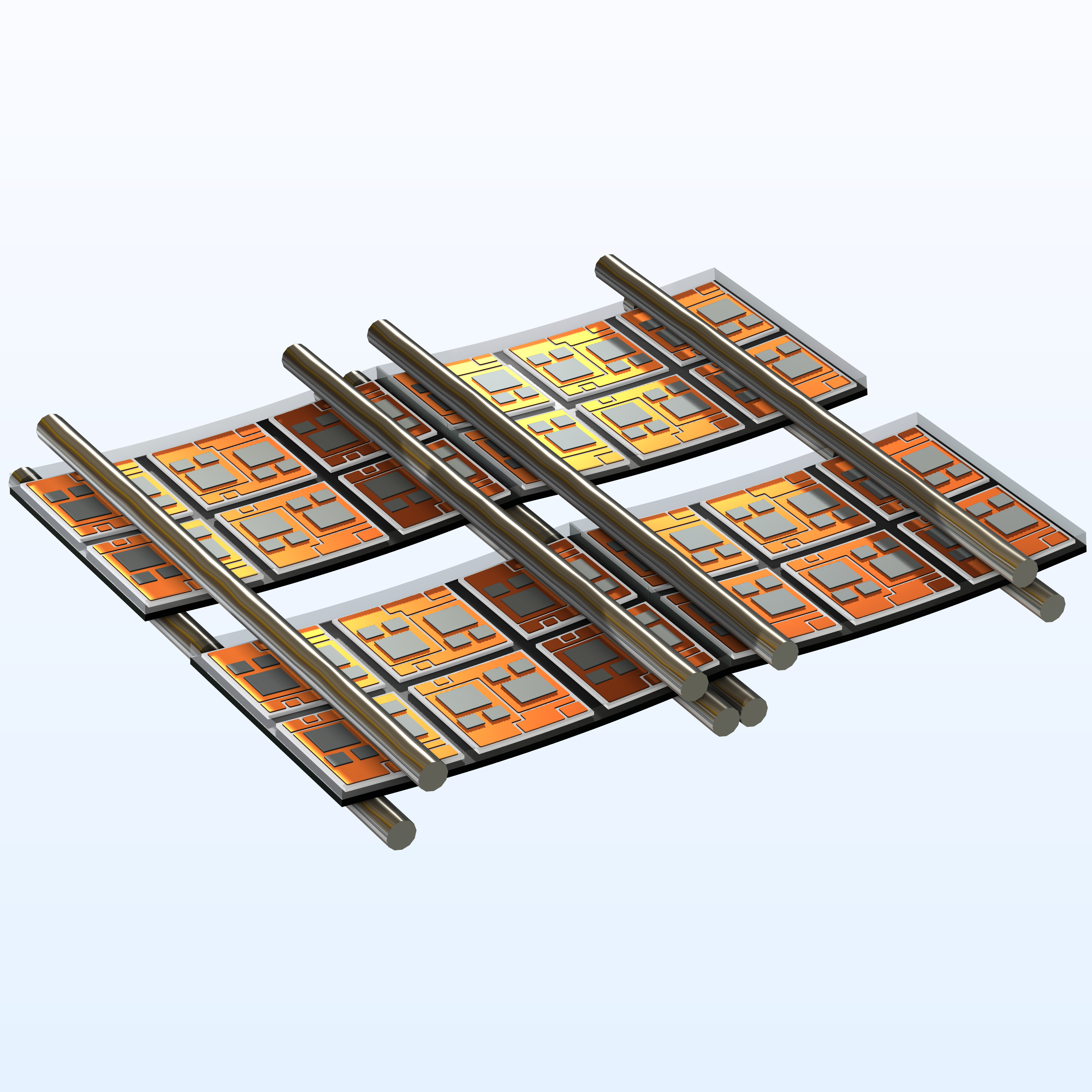 An IGBT module model visualized to be mirrored and in a 2x2x1 array to create a more complex geometry of multiple modules.
An IGBT module model visualized by using the Array 3D dataset to create a 2x2x1 array of the previous Mirror 3D dataset to create a larger geometry appearance.
An IGBT module model visualized to be mirrored and in a 2x2x1 array to create a more complex geometry of multiple modules.
An IGBT module model visualized by using the Array 3D dataset to create a 2x2x1 array of the previous Mirror 3D dataset to create a larger geometry appearance.
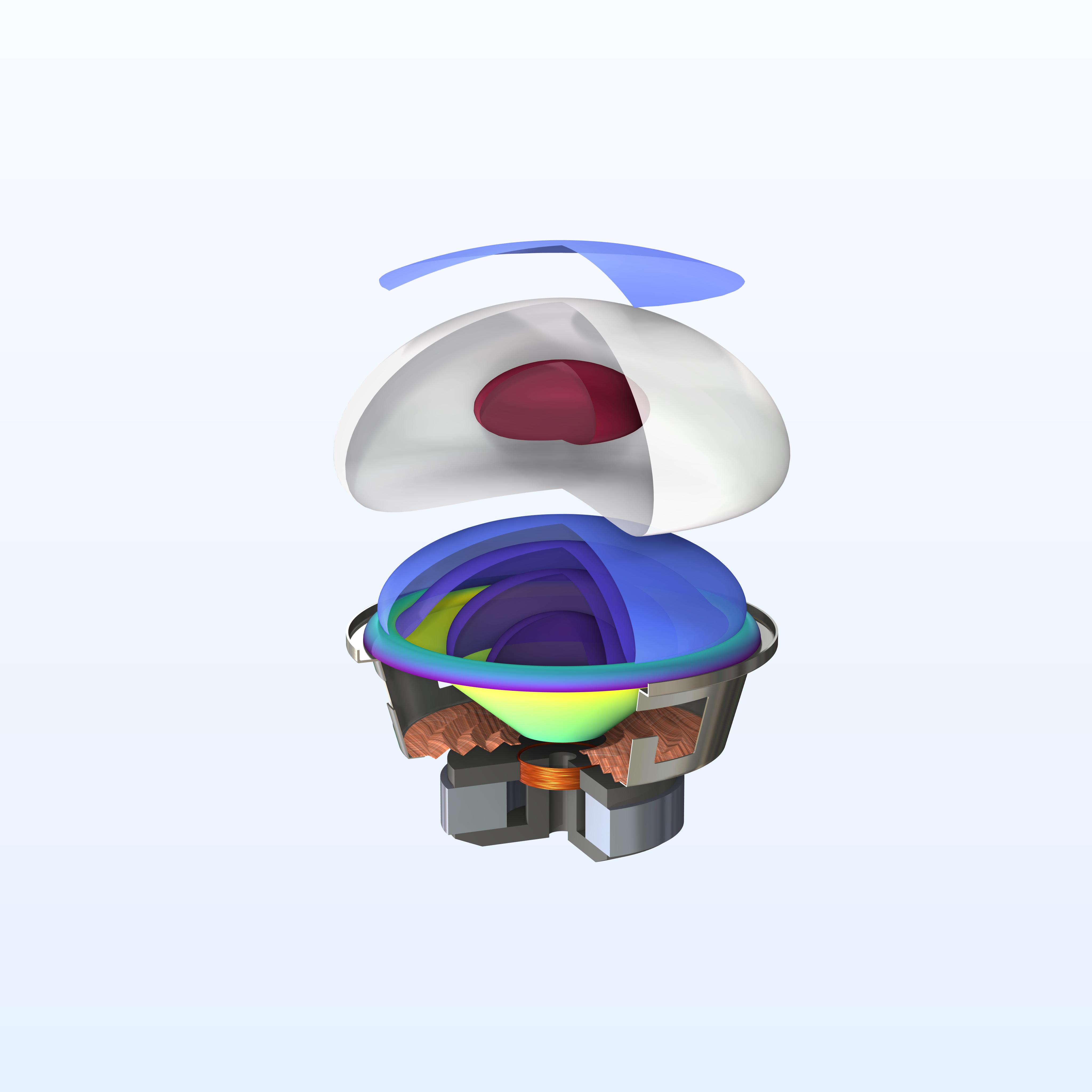
Revolution 1D and 2D datasets and Sector 2D and 3D datasets are useful for models where the initial geometries have been simplified using symmetry to decrease computational time, but the resulting plots need to be visualized in their original full geometry. The Revolution datasets can be used to visualize an axisymmetric model: a 1D model in a 2D space or 2D model in a 3D space, respectively. You can choose the starting angle for the revolved model as well as the full revolution angle and designate whether the dataset will use end caps to close the revolved geometry if the revolution angle value is less than 360°. The Sector 2D and Sector 3D datasets work similarly to plot the solution for the full geometry by exploiting sector symmetries in your model and mirroring or rotating the model accordingly. For each of these datasets, you can make selections to specify the parts of the geometry you would like to revolve. You can see the result of using the Sector 3D dataset on the Loudspeaker Driver in 3D — Frequency-Domain Analysis model below.
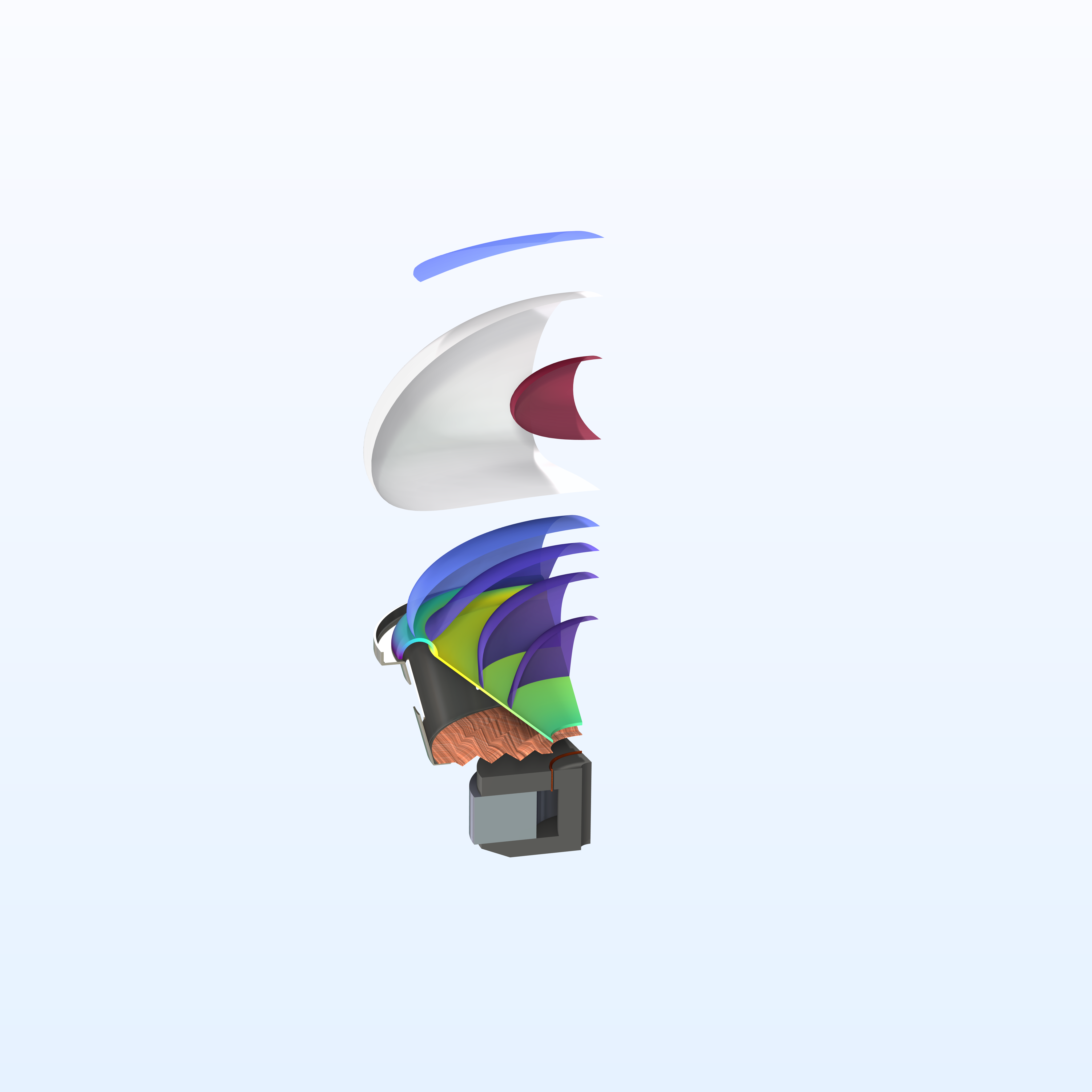 A loudspeaker model visualized with its original solution that is equal to a quarter of its full geometry.
A loudspeaker model visualized with the preset Solution dataset. To save computational costs, this model was created and solved using a quarter of its normal geometry.
A loudspeaker model visualized with its original solution that is equal to a quarter of its full geometry.
A loudspeaker model visualized with the preset Solution dataset. To save computational costs, this model was created and solved using a quarter of its normal geometry.
 A loudspeaker model visualized using multiple Sector 3D datasets to revolve the initial geometry and create the full desired image.
A loudspeaker model visualized using multiple Sector 3D datasets to revolve the initial quartered model geometry and solution to create a more cohesive result appearance.
A loudspeaker model visualized using multiple Sector 3D datasets to revolve the initial geometry and create the full desired image.
A loudspeaker model visualized using multiple Sector 3D datasets to revolve the initial quartered model geometry and solution to create a more cohesive result appearance.
By default, each plot within a plot group uses the dataset designated by the parent plot group node. However, different datasets can be used for each plot within the same plot group to create interesting and complex model visualizations.
Material Appearance
For 2D and 3D plot groups, you can add a Material Appearance feature to certain plot types to further enhance the realistic appearance of a model. This feature can be used to create mixed visualizations, where some plots show the results of the simulation, while others show the geometry of the model, allowing for more complex visual representation. The images below depict the impact of using the Material Appearance functionality on The Epitaxial Growth of SiC by the PVT Method model.
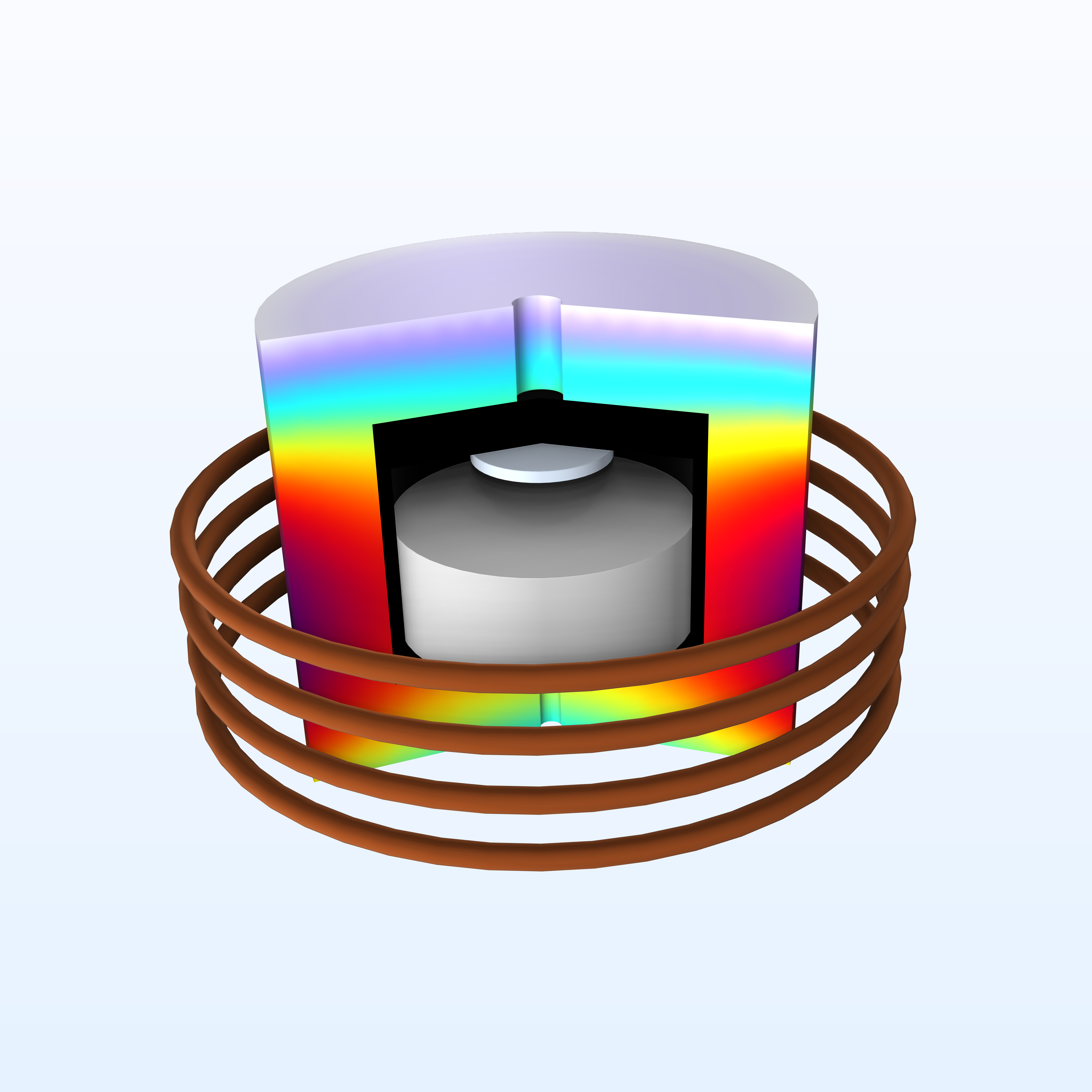 A silicon carbide epitaxial furnace model showing the magnetic flux density norm without using the Material Appearance feature.
A silicon carbide (SiC) epitaxial furnace model visualized without using the Material Appearance feature.
A silicon carbide epitaxial furnace model showing the magnetic flux density norm without using the Material Appearance feature.
A silicon carbide (SiC) epitaxial furnace model visualized without using the Material Appearance feature.
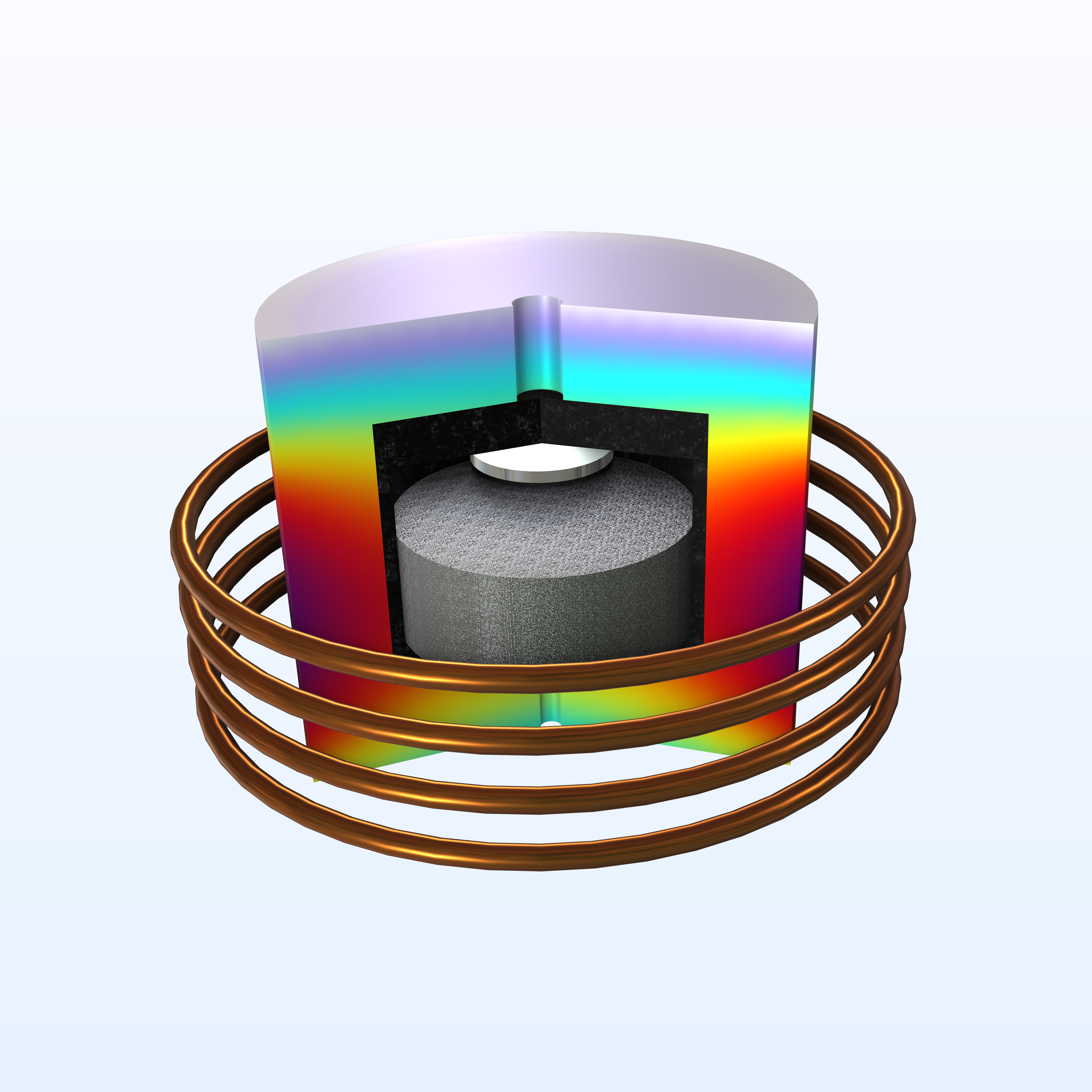 A silicon carbide epitaxial furnace model showing the magnetic flux density norm using various different Material Appearance features.
A silicon carbide (SiC) epitaxial furnace model visualized using the Material Appearance feature.
A silicon carbide epitaxial furnace model showing the magnetic flux density norm using various different Material Appearance features.
A silicon carbide (SiC) epitaxial furnace model visualized using the Material Appearance feature.
To access this feature, right-click the plot type node and select Material Appearance from the list. In the Settings window for Material Appearance , the Appearance menu has two options. The From material option allows for the plot to take on the designated appearance of the material set earlier in the Materials node. The Customize option enables you to alter the plot appearance by using the preset material appearances in the Material type list. Additionally, you can further customize the material appearances from the Material type list by pressing the Customize button and moving each slider accordingly to acquire the desired effect. To use the results of a plot instead of the material’s inherent color, while still maintaining the texture or properties of the material you are visualizing, select the Use the plot’s color checkbox in the Settings window.
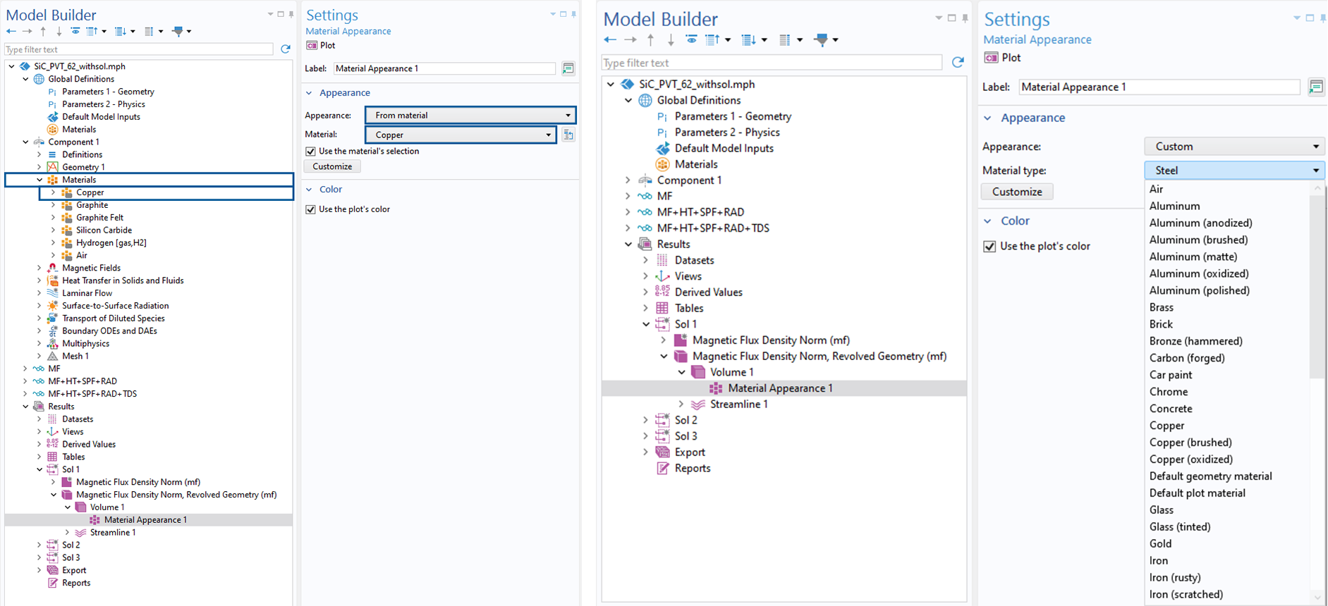 The Material Appearance settings window open and the associated Copper material highlighted beneath the Materials node in the Model Builder tree. (left) The Material Appearance settings window open with the Material type drop down menu showing a list of preset material options. (right)
The Settings window for the Material Appearance feature with the From material option selected and the corresponding Copper material option selected (left) and the Settings window for the Material Appearance feature with the Custom appearance option selected and some of the preset material appearances shown in the Material type list (right).
The Material Appearance settings window open and the associated Copper material highlighted beneath the Materials node in the Model Builder tree. (left) The Material Appearance settings window open with the Material type drop down menu showing a list of preset material options. (right)
The Settings window for the Material Appearance feature with the From material option selected and the corresponding Copper material option selected (left) and the Settings window for the Material Appearance feature with the Custom appearance option selected and some of the preset material appearances shown in the Material type list (right).
Visual Effects
Ambient Occlusion, Direct Shadows, Floor Shadows, and Indoor Environment or Outdoor Environment mapping can all help to add depth and shading in different ways to a model, resulting in a more realistic appearance. They can each be toggled on and off in the Graphics window within the Scene Light menu. Additionally, in the View node under the Definitions node in the Model Builder tree, you can find further settings for the visual effects already noted, as well as different individual lighting settings.
 A close-up of the Scene Light menu located within the Graphics window, with the ambient occlusion, direct shadows, floor shadows, outdoor environment, and environment reflections toggled (left). The Model Builder tree with the View node highlighted and its corresponding Settings window open right).
Scene Light menu located within the Graphics window (left) and the Settings window for the View node.
A close-up of the Scene Light menu located within the Graphics window, with the ambient occlusion, direct shadows, floor shadows, outdoor environment, and environment reflections toggled (left). The Model Builder tree with the View node highlighted and its corresponding Settings window open right).
Scene Light menu located within the Graphics window (left) and the Settings window for the View node.
Ambient Occlusion is a rendering technique used to simulate the soft shadows and shading effects that arise from ambient lighting in a scene. It enhances the perception of depth and detail by darkening areas where surfaces are close to each other, such as holes, creases, and edges, where light would naturally be occluded. The Direct Shadows option, on the other hand, simulates shadows cast by objects within the geometry as a result of direct illumination from specific light sources. This technique provides more defined shadows, contributing to the realism of the rendering. Direct Shadows can be used individually or together with Ambient Occlusion to further improve the realism of model geometries or plots. The Floor Shadows option must be used together with either the Ambient Occlusion or the Direct Shadows option in order for it to appear. The floor shadow that appears is dependent on which shadow rendering technique is being used; use it together with Ambient Occlusion for a light shadow beneath the geometry on the model floor, or use it with Direct Shadows for a heavier shadow that depicts a more in-depth view of the model geometry. All three of these shadow rendering techniques can be used at once for further realistic visualization, and the shadow strength, softness, and quality settings for each can be further altered and customized from the View node.
The Indoor Environment and Outdoor Environment options enable you to enhance the reflections of a texture created using the Material Appearance feature. Only one environment option can be toggled on at a time. This appearance setting becomes particularly useful for more reflective textures such as chrome, steel, or aluminum (polished), as it allows for a more realistic reflection on the model geometry. In the Environment Settings window for the View node, you can also choose from which axis the sky direction is depicted, as well as rotate the environment around to create different reflections. In some cases, you may also want to view the environment background or use it for the image background and can do so by toggling on the Skybox feature. Below you can see the effect of utilizing these visual techniques on the Analysis of NOx Reaction Kinetics model.
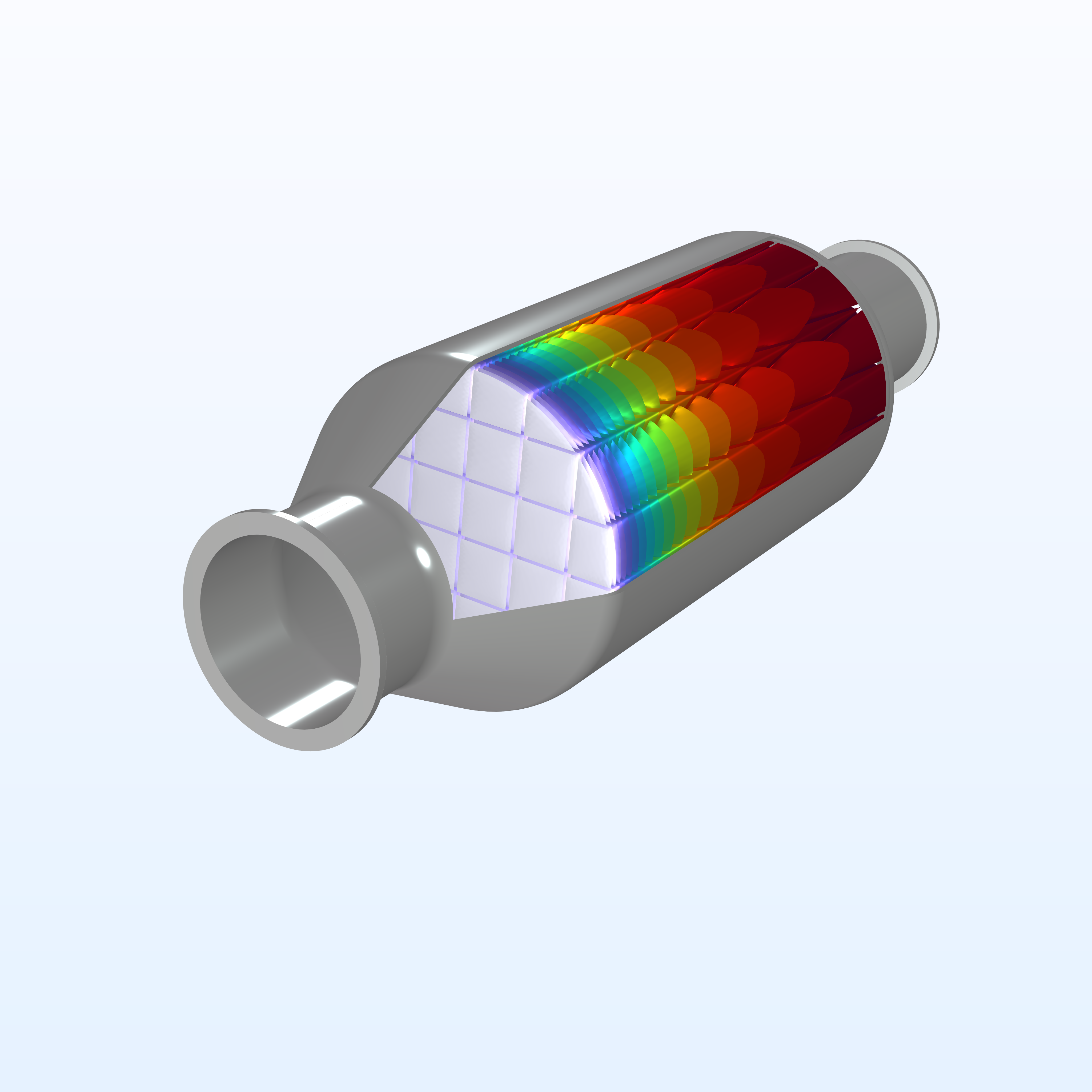 A monolith reactor model showing the species transport flow rate without any shadow or environment rendering added to it.
A monolith reactor model visualized without using shadow or environment rendering.
A monolith reactor model showing the species transport flow rate without any shadow or environment rendering added to it.
A monolith reactor model visualized without using shadow or environment rendering.
 A monolith reactor model showing the species transport flow rate with shadow and environment rendering added.
A monolith reactor model visualized using the Ambient Occlusion, Direct Shadows, Floor Shadows, and Indoor Environment features.
A monolith reactor model showing the species transport flow rate with shadow and environment rendering added.
A monolith reactor model visualized using the Ambient Occlusion, Direct Shadows, Floor Shadows, and Indoor Environment features.
 A sports car model showing the velocity field without any shadow or environment rendering added to it.
A sports car model visualized without using shadow or environment rendering.
A sports car model showing the velocity field without any shadow or environment rendering added to it.
A sports car model visualized without using shadow or environment rendering.
 A sports car model showing the velocity field visualized using various shadow features, environment rendering, and the skybox.
A sports car model visualized using the Ambient Occlusion, Direct Shadows, and Outdoor Environment features with the Skybox toggled on and blurred in the background.
A sports car model showing the velocity field visualized using various shadow features, environment rendering, and the skybox.
A sports car model visualized using the Ambient Occlusion, Direct Shadows, and Outdoor Environment features with the Skybox toggled on and blurred in the background.
Scene Lighting and Camera Views
For 3D models, there are Directional Light, Point Light, Spotlight, and Headlight options that can be used to customize the lighting, coloring, and shading of your model. By default, each view comes with three Directional Light sources, but can have up to a maximum of eight light source nodes in total. For each of the light sources, you can adjust the color, light intensity, and specular intensity to achieve the desired lighting or shading of your model. Directional Lights act almost like sunlight rays on an object, where the corresponding light will fall on all of the objects in its direction. The direction of the light can be changed by adjusting the values of the x, y, and z coordinates. Point Lights have a specific position and act as a lightbulb on an area of your model and can be adjusted just like a Directional Light. The Spotlight option acts like a flashlight turned onto the model, and the spread angle of the light can be adjusted along with the position and direction. The Headlight option is a larger directional light that points solely from the camera’s position and is locked to the camera’s own coordinate system.
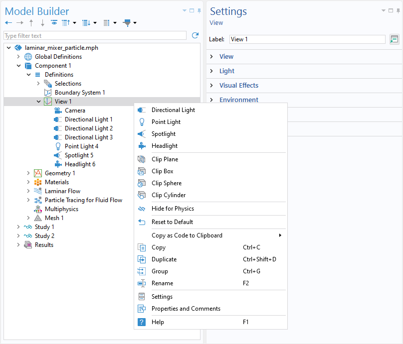 The Model Builder tree with the View node highlighted and its corresponding menu open to show the different light sources to choose from.
The different light source options listed within the View node menu.
The Model Builder tree with the View node highlighted and its corresponding menu open to show the different light sources to choose from.
The different light source options listed within the View node menu.
For finishing touches on your image, you can add a more dynamic camera view by holding the Alt key and zooming in or out from your model in the Graphics window to activate the mouse dolly. This keeps the model in the center of the camera view but angles the lens to give an interesting fish-eye lens perspective of your model. Additionally, to better manipulate your model into more dynamic views, a 3Dconnexion SpaceMouse® can be especially beneficial. To remove the model's geometry lines for a more seamless image appearance, deselect the Plot dataset edges option in the plot group Settings window.
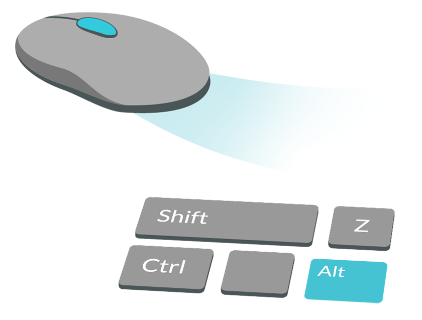
Infographic depicting how to activate the mouse dolly camera.
Exporting Your Model Image
To export high-quality images, press the Image Snapshot button in the Graphics window toolbar and adjust your settings to export a 4096 x 4096 pixel (px) image with a resolution of 300 DPI on a transparent background. The Antialiasing option should always be checked, whereas the Zoom extents option should only be checked when necessary. Please note that 4096 x 4096 px is the maximum size an image snapshot can be.
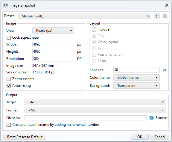
The Image Snapshot window with the appropriate settings to produce a high-quality image.
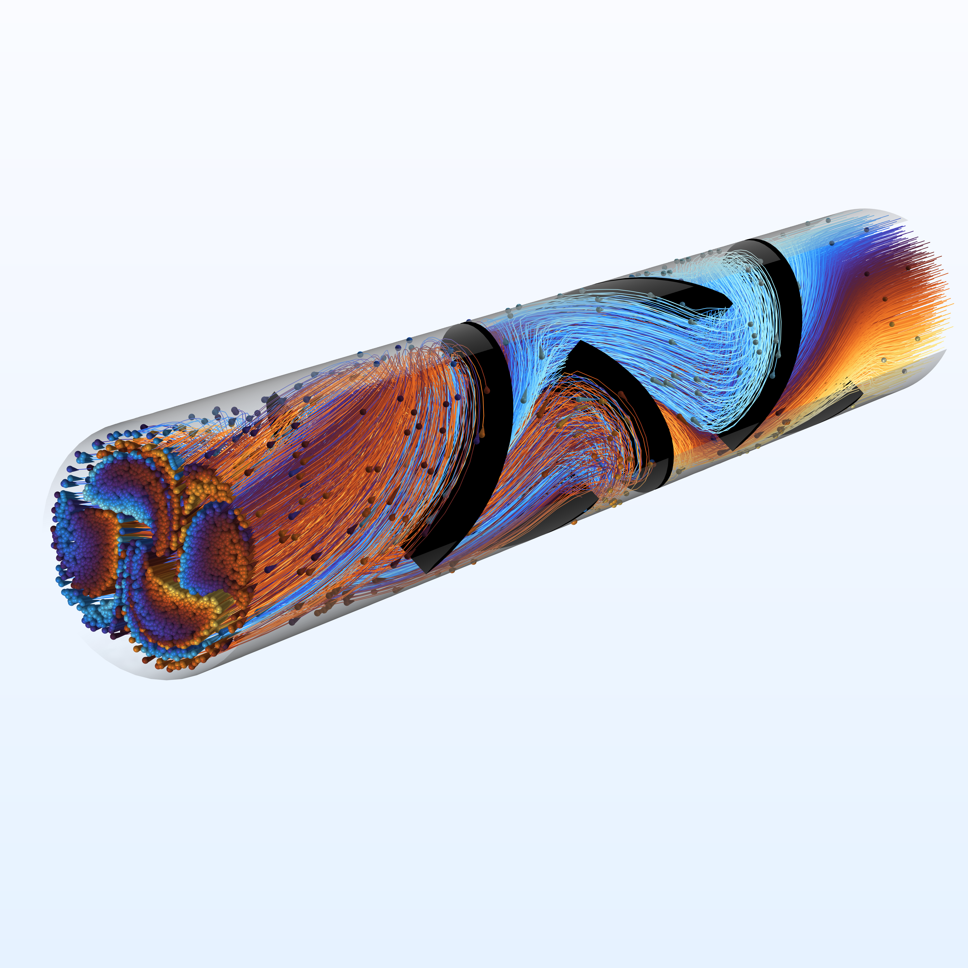 A laminar static mixer model showing the particle trajectories without using any lighting or camera view techniques.
A static mixer model visualized without using the mouse dolly or lighting techniques.
A laminar static mixer model showing the particle trajectories without using any lighting or camera view techniques.
A static mixer model visualized without using the mouse dolly or lighting techniques.
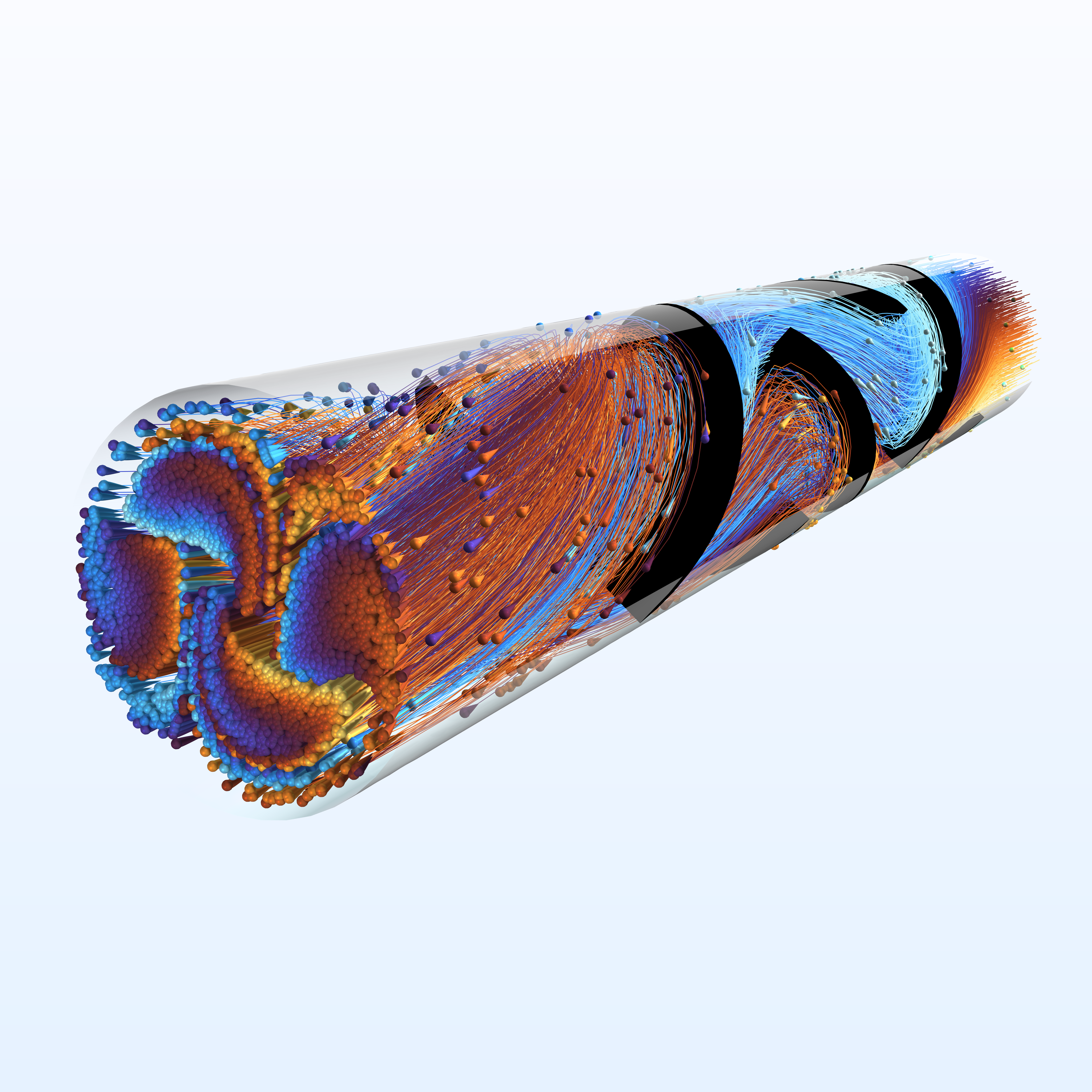 A laminar static mixer model showing the particle trajectories using the mouse dolly camera view and various lighting techniques.
A static mixer model visualized using the mouse dolly camera view and lighting techniques.
A laminar static mixer model showing the particle trajectories using the mouse dolly camera view and various lighting techniques.
A static mixer model visualized using the mouse dolly camera view and lighting techniques.
Demo: Generating High-Quality Model Images
In the following video, we use the Large Eddy Simulation of a Sports Car to summarize all of the strategies outlined above to show the impact they can make on a model when used together from beginning to end.
Submit feedback about this page or contact support here.