Starting to Model Magnetohydrodynamics
Over the next five parts of the course, we will discuss how to set up each part of a magnetohydrodynamic (MHD) model, including the geometry, materials, physics interfaces, couplings, mesh, and solver configurations. The main part of each section will present how to perform a variety of different, common techniques that are required for modeling MHD in the COMSOL® software.
This part begins with an introduction to the first steps in creating an MHD model:
- Adding the magnetohydrodynamics physics to the model
- Deciding on a modeling domain and creating the geometry for it
- Adding the material properties
- Choosing whether to use a one-way or two-way version of a magnetohydrodynamics coupling
- Choosing a study type to solve the physics
We will also present a series of exercises that demonstrate how these techniques are used in practice within the context of common MHD applications. The four systems used as example are a magnetohydrodynamic pump, a rotational velocity measurement device, Hartmann flow in a 3D duct, and a uniform flow in a pipe with finite conductivity in a transverse magnetic field.
Adding the Magnetohydrodynamics Physics
The Select Physics menu in the Model Wizard and the Add Physics menu, accessed by using the Add Physics button in the ribbon, both allow the Laminar Flow interface and the appropriate electromagnetic physics interface to be added to the model together with the Magnetohydrodynamics multiphysics coupling. The physics are added through the following path in the menus: AC/DC > Electromagnetics and Fluids. From there, if a 3D component is being used, you should select the Magnetohydrodynamics interface. If a 2D cross section or 2D axisymmetric component is being used, you can choose from the following options:
- The Magnetohydrodynamics, Out-of-Plane Currents option, which will add the Magnetic Fields interface as the electromagnetics interface
- The Magnetohydrodynamics, In-Plane Currents option, which will add the Magnetic and Electric Fields interface as the electromagnetics interface
This method allows the correct interface for the currents to be chosen.
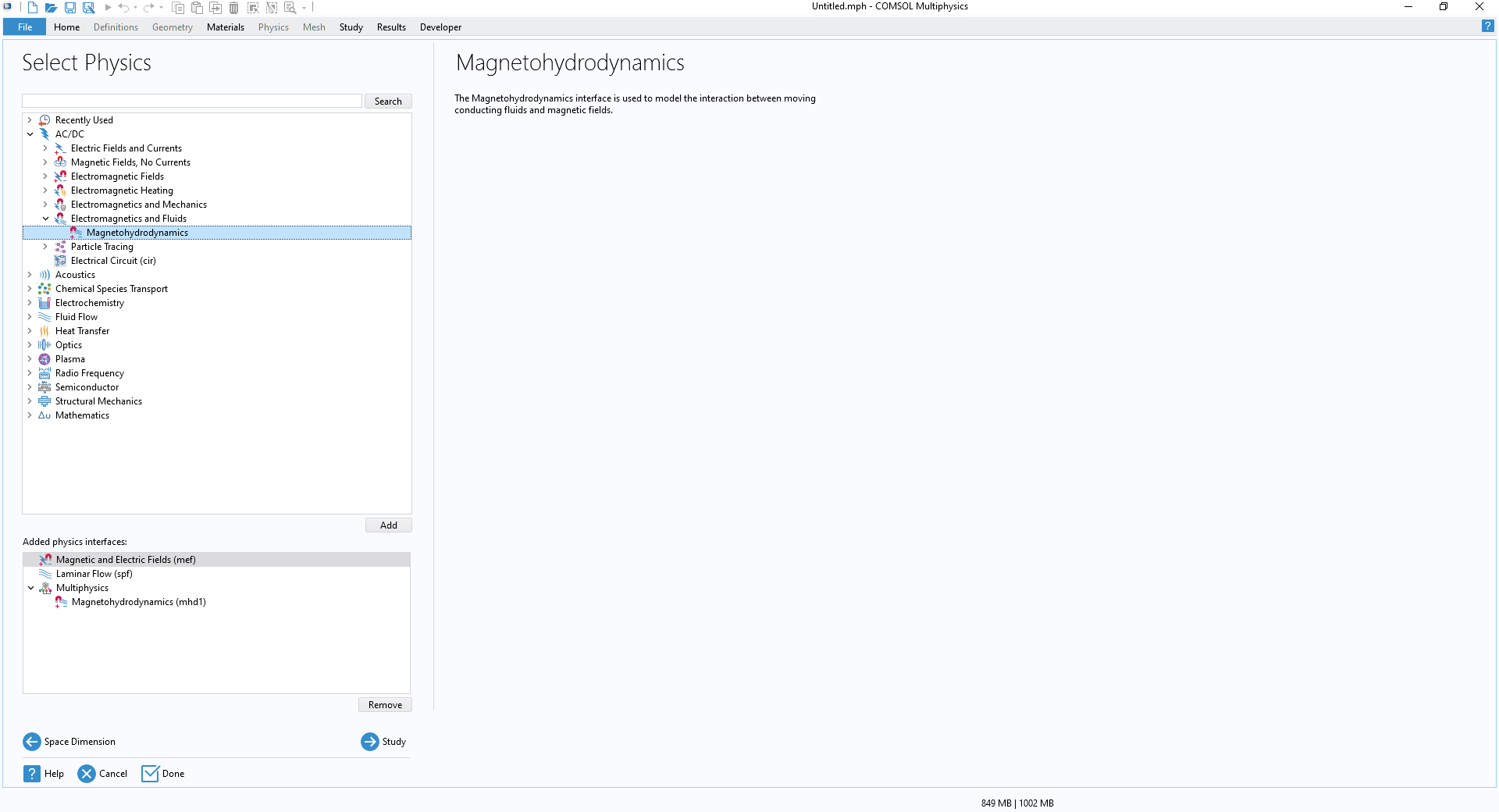 The COMSOL Multiphysics Select Physics interface with the Magnetohydrodynamics multiphysics interface selected.
The Select Physics menu for a 3D component in the Model Wizard, showing the Magnetohydrodynamics multiphysics interface in the menu as well as the added Magnetic and Electric Fields and Laminar Flow interfaces and Magnetohydrodynamics coupling.
The COMSOL Multiphysics Select Physics interface with the Magnetohydrodynamics multiphysics interface selected.
The Select Physics menu for a 3D component in the Model Wizard, showing the Magnetohydrodynamics multiphysics interface in the menu as well as the added Magnetic and Electric Fields and Laminar Flow interfaces and Magnetohydrodynamics coupling.
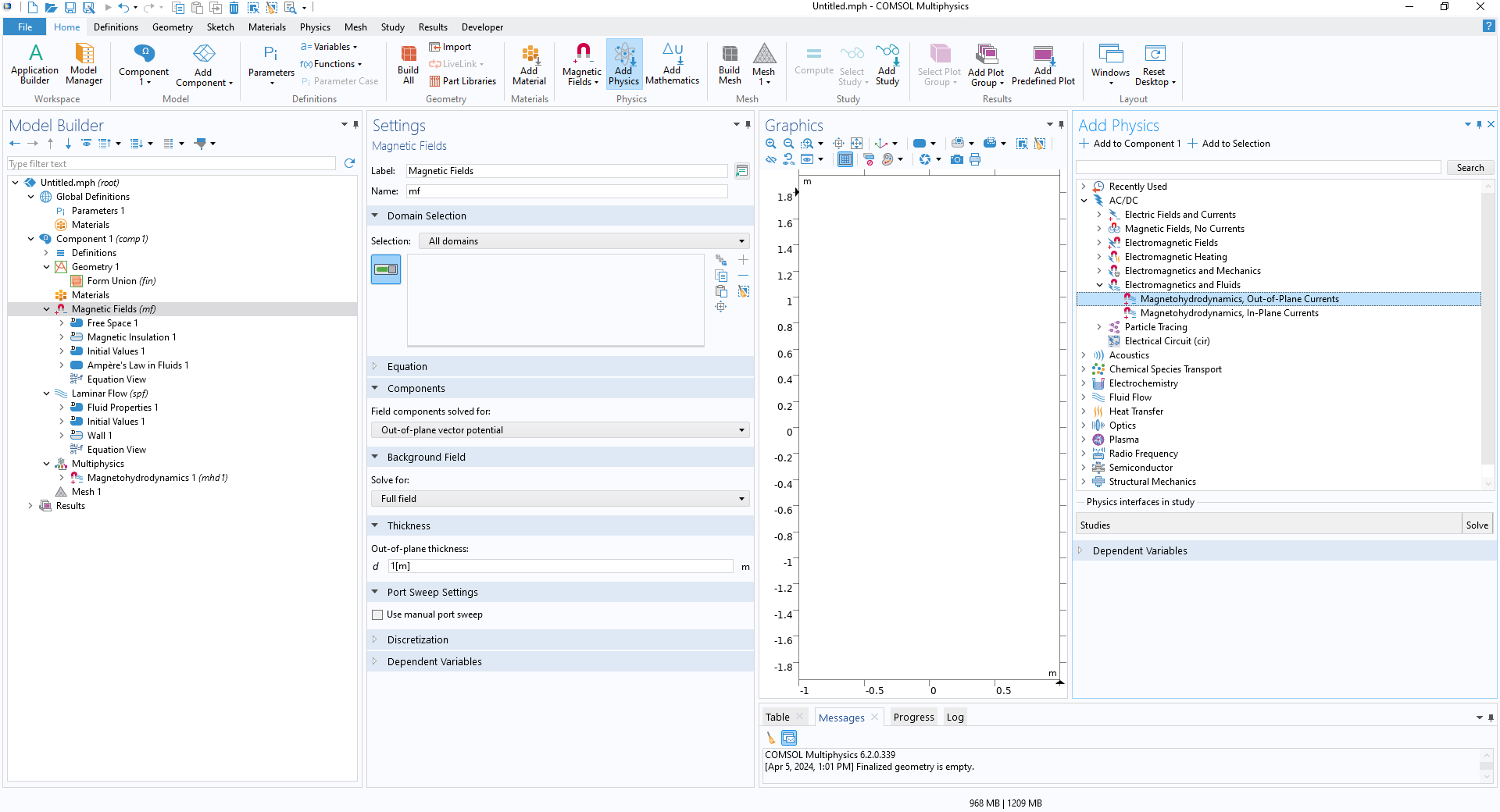 COMSOL Multiphysics with the Add Physics menu open and the Magnetohydrodynamics, Out-of-Plane Currents option selected.
The Add Physics menu in a model with a 2D component was used to select the Magnetohydrodynamics, Out-of-Plane Currents option and add the Magnetic Fields and Laminar Flow interfaces with the Magnetohydrodynamics coupling.
COMSOL Multiphysics with the Add Physics menu open and the Magnetohydrodynamics, Out-of-Plane Currents option selected.
The Add Physics menu in a model with a 2D component was used to select the Magnetohydrodynamics, Out-of-Plane Currents option and add the Magnetic Fields and Laminar Flow interfaces with the Magnetohydrodynamics coupling.
By using the multiphysics interface, additional adjustments to the default settings in the electromagnetics interface are automatically made when the electromagnetics interface is added to the model. This makes the electromagnetics interface more suitable for performing MHD flow modeling.
Choosing the Study
The physics interface sets the general equation that will be solved in the model, but the formulation of this equation (stationary, transient, or Fourier transformed into the frequency domain) is set in the study step where the interface is solved.
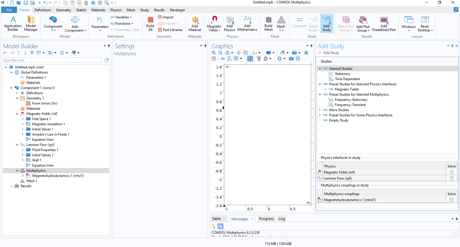 COMSOL Multiphysics with the Add Study menu open, with the Stationary, Time Dependent, Frequency-Stationary, and Frequency-Transient options displayed.
The Add Study menu for a model with a Magnetohydrodynamics coupling, showing the Stationary and Time Dependent study steps in the General Studies section and the Frequency-Stationary and Frequency-Transient study steps in the Preset Studies for Selected Multiphysics section.
COMSOL Multiphysics with the Add Study menu open, with the Stationary, Time Dependent, Frequency-Stationary, and Frequency-Transient options displayed.
The Add Study menu for a model with a Magnetohydrodynamics coupling, showing the Stationary and Time Dependent study steps in the General Studies section and the Frequency-Stationary and Frequency-Transient study steps in the Preset Studies for Selected Multiphysics section.
The Stationary study is designed to identify an equilibrium solution. When exciting the model with a current, it is suitable for the case of a constant DC current.
The Time Dependent study is designed for cases where determining the transient behavior of a system is required. Reasons why computing transient behavior might be required are that there is no equilibrium solution, the loads of the system are transient, or that studying the transient development is needed in the design process at hand.
The solver in the time-dependent study will match the length of the solver time steps to the rate of change of the solution. If the electromagnetic fields change on a time scale several orders of magnitude faster than the fluid flow — for example, because the system is loaded using coils driven with an AC current working at tens to thousands of Hertz — then the time steps will have a maximum length that corresponds to the electromagnetic time scale, several orders of magnitude smaller than the fluid flow's time scale. This can require very large numbers of time steps to see any evolution in the flow and can be very computationally expensive.
In the case where the rapid change in electromagnetic problem is due to the system operating with an oscillating field or current — an AC excitation at a fixed frequency — this can be mitigated by working with the Frequency-Stationary or Frequency-Transient study step. These steps solve the electromagnetic problem in the frequency domain and then use the cycle-averaged values to calculate the stationary or transient fluid flow, respectively. This split formulation is computationally efficient. For the Frequency-Transient excitation, it is also possible to have a source operating at a fixed frequency that has a time-dependent amplitude.
When one of the study steps working in the frequency domain is added to the model, the operating frequency for the model is set in the study step, and the expressions used to define boundary conditions and loads or sources in the electromagnetics interface are then the amplitudes for the oscillating system.
 The Frequency-Stationary study Settings window and selected Physics and Multiphysics couplings are shown.
A magnetohydrodynamic pump. The operating frequency is set at 50 Hz in the Frequency-Stationary study step.
The Frequency-Stationary study Settings window and selected Physics and Multiphysics couplings are shown.
A magnetohydrodynamic pump. The operating frequency is set at 50 Hz in the Frequency-Stationary study step.
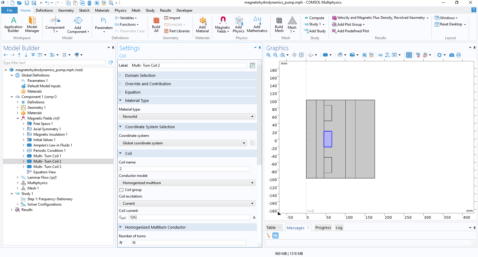 The Settings window for a coil node showing the material type, coordinate system selection, coil name, conductor model, current, and the number of turns.
In the Coil node, the current is set to have an amplitude of 1A, resulting in it being driven with a current equal to 1[A]*sin(2*pi*t*50[Hz]) in the time domain.
The Settings window for a coil node showing the material type, coordinate system selection, coil name, conductor model, current, and the number of turns.
In the Coil node, the current is set to have an amplitude of 1A, resulting in it being driven with a current equal to 1[A]*sin(2*pi*t*50[Hz]) in the time domain.
Defining the Parameters
The Parameters node can be used to define the parameters used to set up the model. For MHD models, the feature provides a useful way to calculate the dimensionless numbers, which you can then use to determine if the model is in the expected flow and electromagnetic regimes. This includes the Reynolds number, magnetic Reynolds number, and Hartmann number.
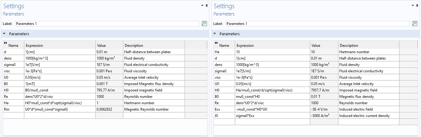 The Parameters settings showing all of the configured parameters with a name, expression, value, and description.
The Parameters node is used to define material properties for the fluid, the characteristic length and velocity of the problem, and the background magnetic field so that the Reynolds number, Hartmann number, and magnetic Reynolds number can be calculated (left). The Hartmann number is specified and used to calculate an appropriate background magnetic flux density for the model (right).
The Parameters settings showing all of the configured parameters with a name, expression, value, and description.
The Parameters node is used to define material properties for the fluid, the characteristic length and velocity of the problem, and the background magnetic field so that the Reynolds number, Hartmann number, and magnetic Reynolds number can be calculated (left). The Hartmann number is specified and used to calculate an appropriate background magnetic flux density for the model (right).
Defining the Geometry
In the Geometry node, the geometry defining the system can either be created in COMSOL® or imported via the CAD Import Module or one of the LiveLink™ for CAD products.
For most MHD models, the volume of the fluid; the volume of the walls enclosing the fluid; any coils, magnets, and leads; and surrounding air must each be defined as a domain. The geometry will then be fully defined.
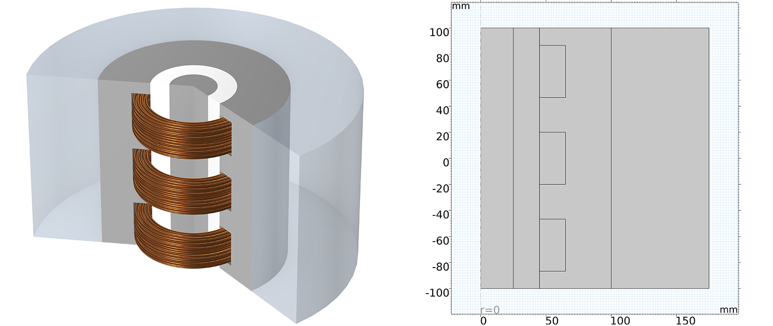
The geometry used for the Magnetohydrodynamics Pump model. Left: schematic of the system showing the combination of coils, the iron structure, the fluid channel filled with liquid lithium, and the surrounding air. Right: The geometry shown as a 2D axisymmetric model.
Reducing the Modeling Domain — Flow in Uniform Background Field
As we will see in three of the model examples in this course, a common magnetohydrodynamics problem will include flow of liquid metal or another conductive fluid in a duct, pipe, or channel; between plates; or within some other container within a uniform background magnetic field. The physical setup of these types of systems is very simple: a fluid volume enclosed by walls and with an air domain surrounding the walls.
The boundary condition that is used to apply the uniform background magnetic field in the Magnetic and Electric Fields interface is able to set the boundary it is applied to as a perfect insulator or a perfect conductor. This can be used to reduce what geometry needs to be included in the modeling domain. For instance:
If the walls of the container have finite conductivity, the air domain can be excluded from the modeling domain. The boundary condition defining the field will be applied to the external boundary of the walls, setting them as in contact with a perfect electric insulator in order to replace the air domain. Only geometry for the fluid volume and container walls is required. If the walls of the container are perfectly insulating or perfectly conducting, then the boundary condition for the background field can be applied to the external boundaries of the fluid. Only geometry for the fluid volume is required.
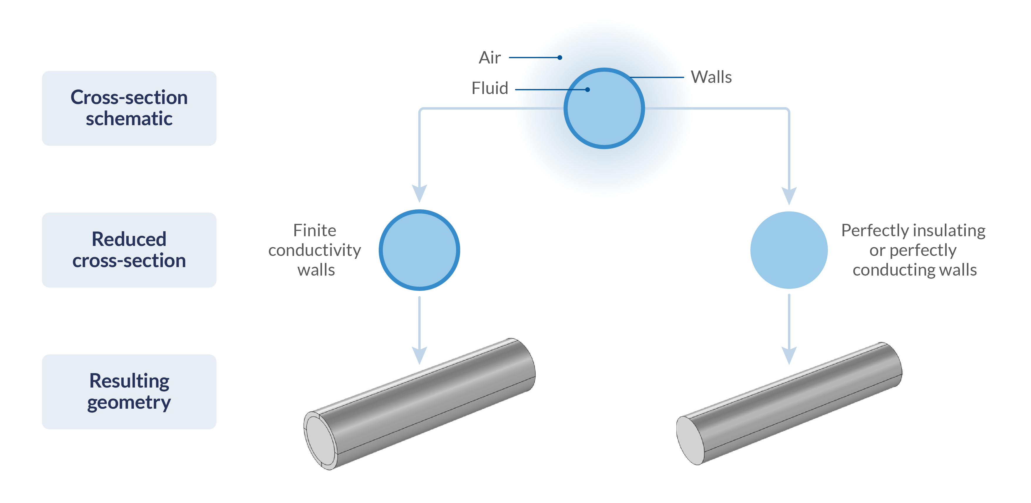
Identifying the geometry required to model flow in a circular pipe surrounded by air in a uniform background field. A representation of the geometry of the cross section of the system (top). The equivalent system cross section once the reduction in the required geometry has been made, for the case of finite thickness, finite conductivity walls (middle left), and the case where the walls are a combination of perfectly insulating and perfectly conducting (middle right). The resulting geometries in COMSOL® (bottom).
Similar reductions in the modeling domain can be made for 2D axisymmetric and cross-section models.
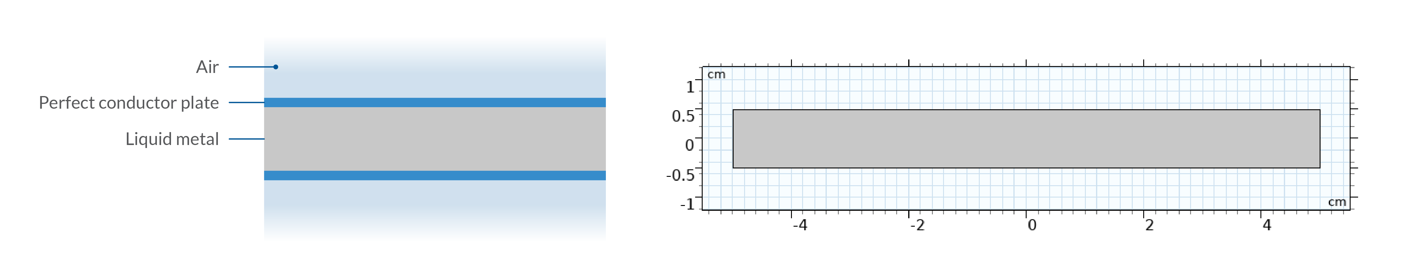
Geometry used to model flow in between infinite plates made of a perfect conductor. The physical system of air, pipe, and liquid metal (left) and the required geometry of only the fluid domain (right).
Setting Material Properties
Once the geometry of the system is defined, materials must be assigned to each of the domains. Materials can either be added by using the Add Material From Library option to access built-in material data sheets or the Add Blank Material option to create a new material, filling out the material properties that are requested. For the fluid, it will be necessary to define the electrical conductivity, relative permittivity, relative permeability, density, and dynamic viscosity.
 COMSOL Multiphysics with the Add Materials menu open and the Sodium-Potassium Eutectic material added.
Using the NaK material from the AC/DC branch > Liquid Metal folder.
COMSOL Multiphysics with the Add Materials menu open and the Sodium-Potassium Eutectic material added.
Using the NaK material from the AC/DC branch > Liquid Metal folder.
When using the Add Material From Library option, the AC/DC branch > Liquid Metals folder in the material database includes these material properties for a number of common liquid metals at a fixed temperature. If the Material Library is available, then the liquid option for the metal materials contains temperature-dependent versions of the electrical conductivity, density, and dynamic viscosity, allowing nonisothermal magnetohydrodynamics modeling once the relative permittivity and permeability are defined and couplings to a heat transfer interface are added.
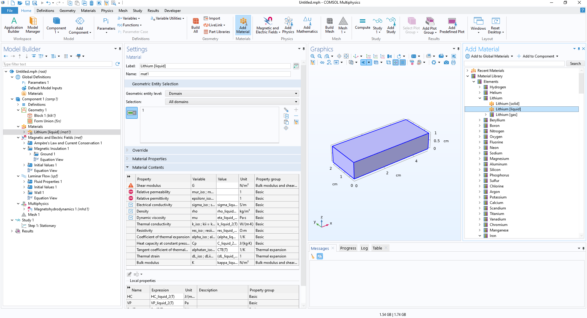 COMSOL Multiphysics with the Add Materials menu open and the Lithium (liquid) material added.
Using the Lithium (liquid) material from the Material Library.
COMSOL Multiphysics with the Add Materials menu open and the Lithium (liquid) material added.
Using the Lithium (liquid) material from the Material Library.
Configuring the Magnetohydrodynamics Coupling
The Magnetohydrodynamics coupling is designed to couple the Laminar Flow interface and one of the suitable electromagnetics interfaces. When added as part of the Magnetohydrodynamics interface, the coupling will automatically have detected the Laminar Flow interface and the electromagnetics interface that were added with it as the two interfaces it is coupling together. The coupling will also be applied to every domain that both the Laminar Flow and electromagnetics interface are applied to — by default, every domain in the model.
The first step in configuring the coupling is to ensure that it is applied only to the domain with the conductive fluid where the magnetohydrodynamic effect will occur. This can be done by clearing the selection for the coupling and reselecting the appropriate domains.
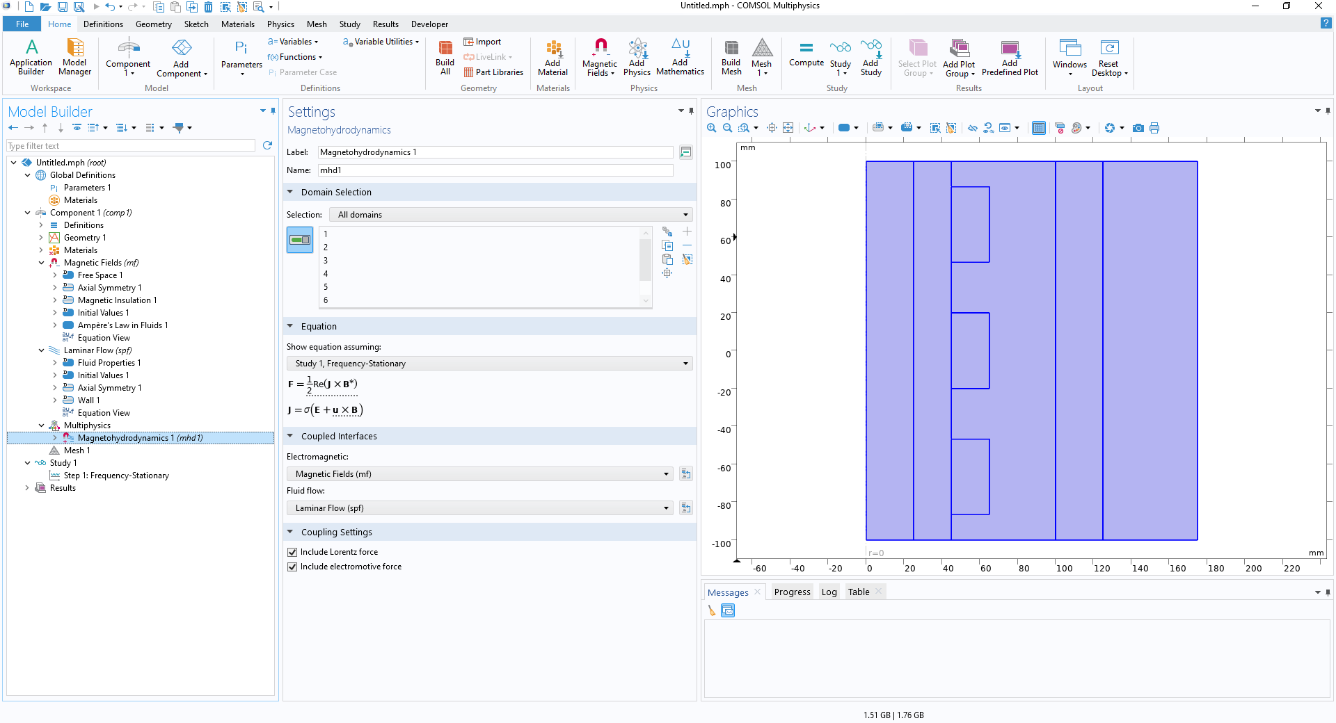 The Magnetohydrodynamic coupling Settings window is shown with the default settings.
The default settings for the Magnetohydrodynamics coupling.
The Magnetohydrodynamic coupling Settings window is shown with the default settings.
The default settings for the Magnetohydrodynamics coupling.
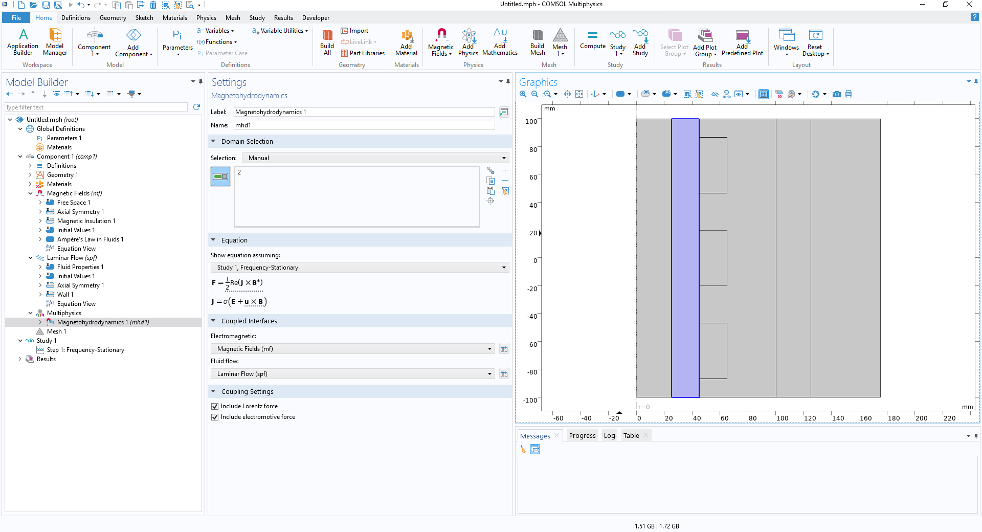 The Magnetohydrodynamic coupling Settings window is shown with the nonliquid metal domains deselected.
All nonliquid metal domains removed from the Magnetohydrodynamics coupling.
The Magnetohydrodynamic coupling Settings window is shown with the nonliquid metal domains deselected.
All nonliquid metal domains removed from the Magnetohydrodynamics coupling.
The coupling between the two interfaces is handled by applying the Lorentz force as a volume force in the Laminar Flow interface, and the current generated by the electromotive force as an external current in the electromagnetics interface.
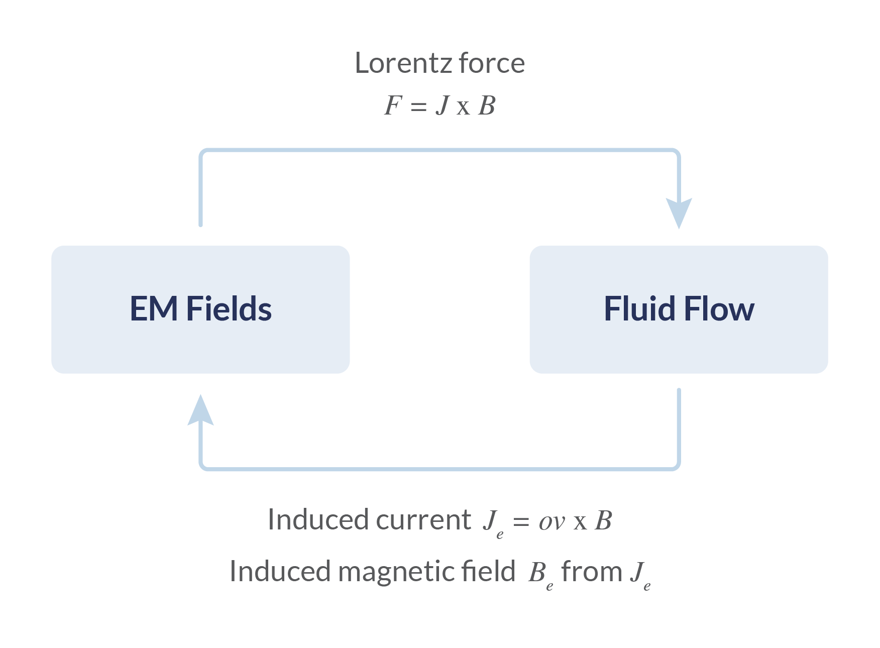
A bidirectional magnetohydrodynamics coupling.
This generates a bidirectional coupling between the two interfaces. This leads to a strongly coupled nonlinear system, as the induced current changes the generated Lorentz force, which changes the fluid velocity, which then changes the induced current, and so on. This can lead to problems that take a long time to compute.
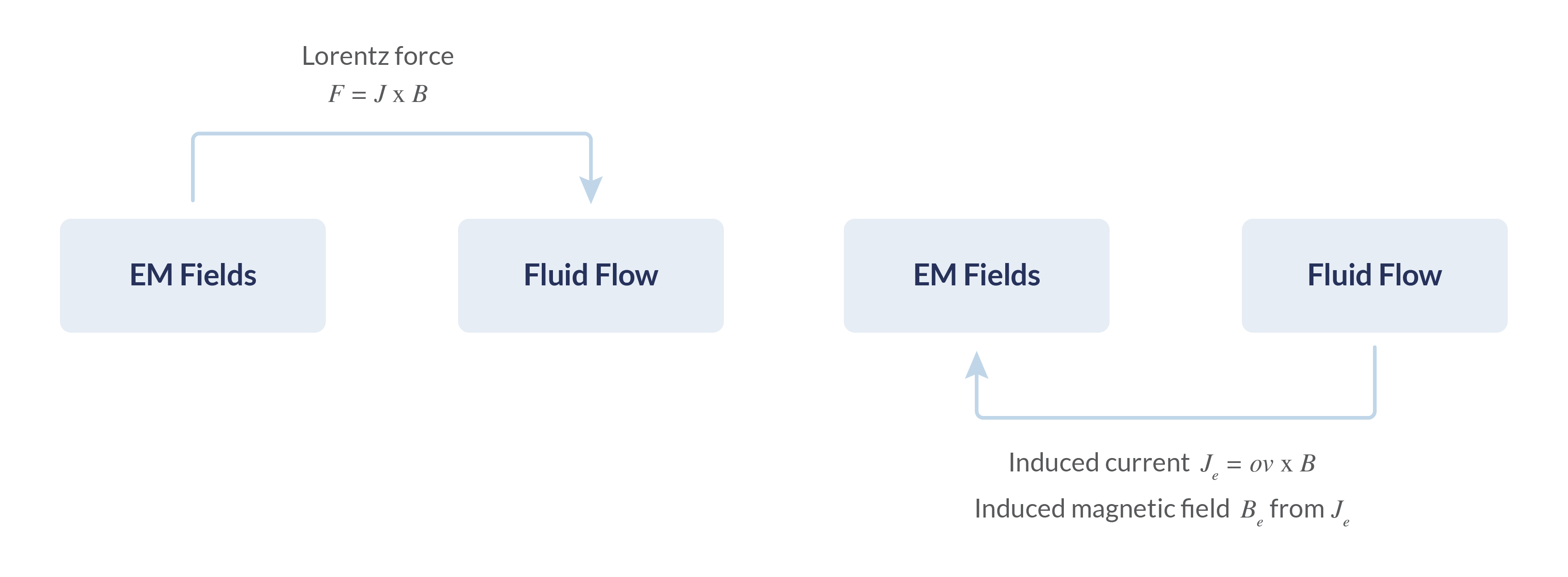
The two possible methods for defining only a one-way-coupled system.
In some cases, it is possible to remove some of the coupling between the two interfaces to decrease the computation time. Each of the Lorentz force and electromotive force contributions can be disabled. Disabling one of these contributions creates a unidirectionally coupled system, which is less nonlinear and easier to solve. The key to deciding whether a coupling can be disabled is determining whether or not including the coupling is the only way the motion of the fluid or the flow of current in the model will occur. In this case, the coupling cannot be disabled.
For an example where creating a one-way coupled system is possible, consider the magnetohydrodynamic pump shown below. The magnetohydrodynamic effect is created by passing a current through the conducting fluid inside the magnetic field of the magnet; the Lorentz force then induces the fluid motion and the pumping effect that is required. Since there is no motion without the Lorentz force, the Lorentz force contribution must be included. However, the current induced by the electromotive force will be negligible compared to the current passed between the two electrodes and can be safely neglected. This allows the electromotive force term to be disabled.

An MHD fluid pump that works by passing a current through the fluid between the two electrodes. Combined with the magnetic field from the magnets, the Lorentz force acts to induce a flow in the pipe. In this system, the electromotive force current is negligible compared to the current due to the potential difference between the electrodes and can be ignored.
On the other hand, a flowmeter, where a conductive fluid passes between two electrodes in a magnetic field and the magnetohydrodynamic effect induces a current between the electrodes, requires the electromotive force term to be enabled. The effect of the Lorentz force on a fast-moving and incompressible fluid may instead be negligible and ignored.
Introducing the Example Models
To apply the techniques discussed in this course, follow along with the examples provided here, which show several common applications for MHD systems: a fluid pump, a motion sensor, and pipe and duct flows.
Magnetohydrodynamics Pump
Induction pumps are used in high-temperature cooling systems. A series of coils surrounding the pipe containing the conductive liquid is driven with an oscillating current with a 120-degree phase shift. This generates eddy currents in the fluid and a resulting Lorentz force that acts to pump the fluid through the pipe. Not requiring any moving parts, and ensuring that the fluid is fully encased, offers significant advantages over other pumping methods. See the Magnetohydrodynamics Pump example model.
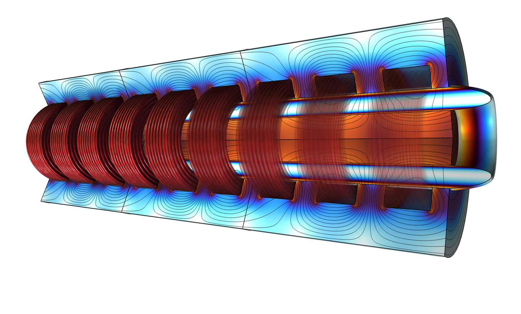
The model demonstrates 2D axisymmetric modeling, out-of-plane currents using the Magnetic Fields interface, the Frequency-Stationary study, and inducing magnetic fields with coils.
Hunt's Case for Flow in a Square Duct
Magnetohydrodynamic flow in a duct within a uniform transverse background magnetic field is a standard problem for testing MHD modeling techniques, as it is both a physically realistic system — transport of a liquid metal in a pipe in a magnetic field — but it is also simple enough to have analytic solutions for certain wall conditions, allowing models to be validated. The HuntFlow_v63.mph model consists of a square duct, placed in a uniform transverse background magnetic field in the z direction, with the flow driven in the x direction by a pressure differential. The vertical walls of the duct parallel to the magnetic field are assumed to be perfectly insulating, while the horizontal walls normal to the field — the Hartmann walls — are perfectly conducting.
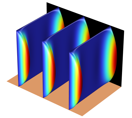
The model demonstrates 3D modeling, applying uniform background fields, using perfectly conducting and insulating walls, symmetry, and periodicity.
Rotational Velocity Meter
Current induced by electromotive force is dependent on the velocity of the fluid. For this reason, one common application of magnetohydrodynamics is to measure the velocity of a fluid by measuring the induced current or potential difference between two electrodes.
A spinning tube and the liquid it is filled with will have the same rotational velocity and acceleration. This demonstrates how the measured potential difference can be used to detect the velocity and acceleration. An example of this relationship is shown in the model RotationalVelocityMeter_v63 and the graph below.
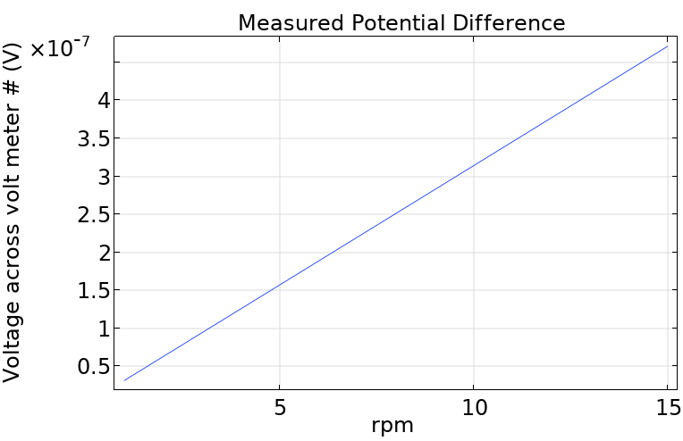
The model demonstrates 2D axisymmetric modeling, in-plane currents using the Magnetic and Electric Fields interface, an azimuthal fluid flow using the swirl flow settings, applying uniform background fields, using perfectly conducting and insulating walls, and connecting the model to an ideal circuit.
Submit feedback about this page or contact support here.