Acoustics Module

Analyze the Acoustics and Vibrations Behavior of Your Products and Designs

Products and designs involving acoustic phenomena can be modeled to study and predict factors like sound quality and noise reduction performance. The Acoustics Module is an add-on to the {:comsolmph] software that provides features for modeling acoustics and vibrations for applications such as speakers, mobile devices, microphones, mufflers, sensors, sonar, flowmeters, rooms, and concert halls. You can visualize These features allow for visualizing acoustic fields and build building virtual prototypes of devices or components.

For more detailed studies, acoustics can be coupled with other physical effects, including structural mechanics, piezoelectricity, and fluid flow. The COMSOL® software includes multiphysics couplings that make it possible to evaluate the performance of a product or design in an environment that is as close as possible to the real world.

The Acoustics Module also includes many specialized formulations and material models, such as for thermoviscous acoustics, used in miniature transducers and mobile devices, or Biot's equations, used for modeling poroelastic waves. The multiphysics environment is extended further with several numerical methods. In addition to the finite element method (FEM), the Acoustics Module features the boundary element method (BEM), the discontinuous Galerkin finite element method (dG-FEM), and ray tracing.

Contact COMSOL
A speaker model showing the interior and exterior sound pressure level in the Prism color table.

Pressure Acoustics

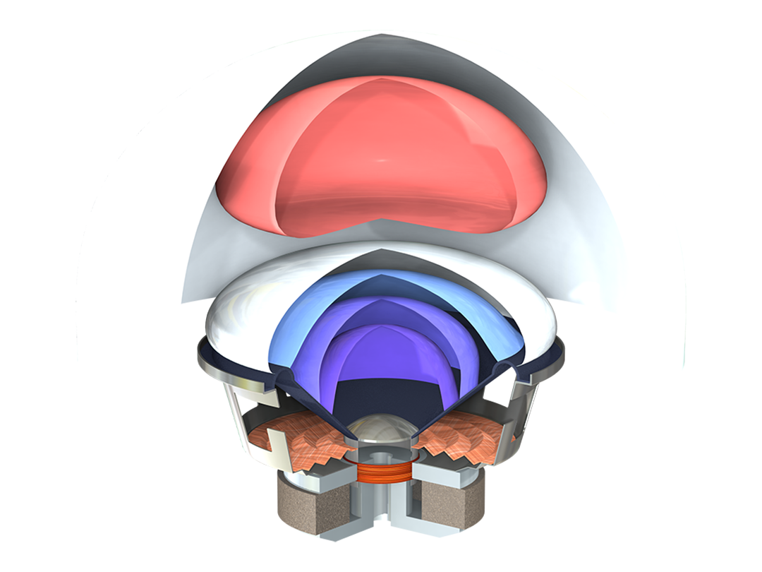
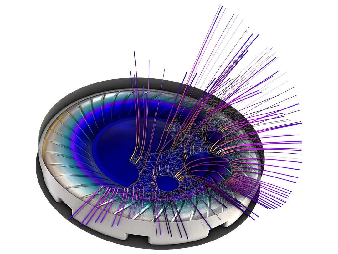
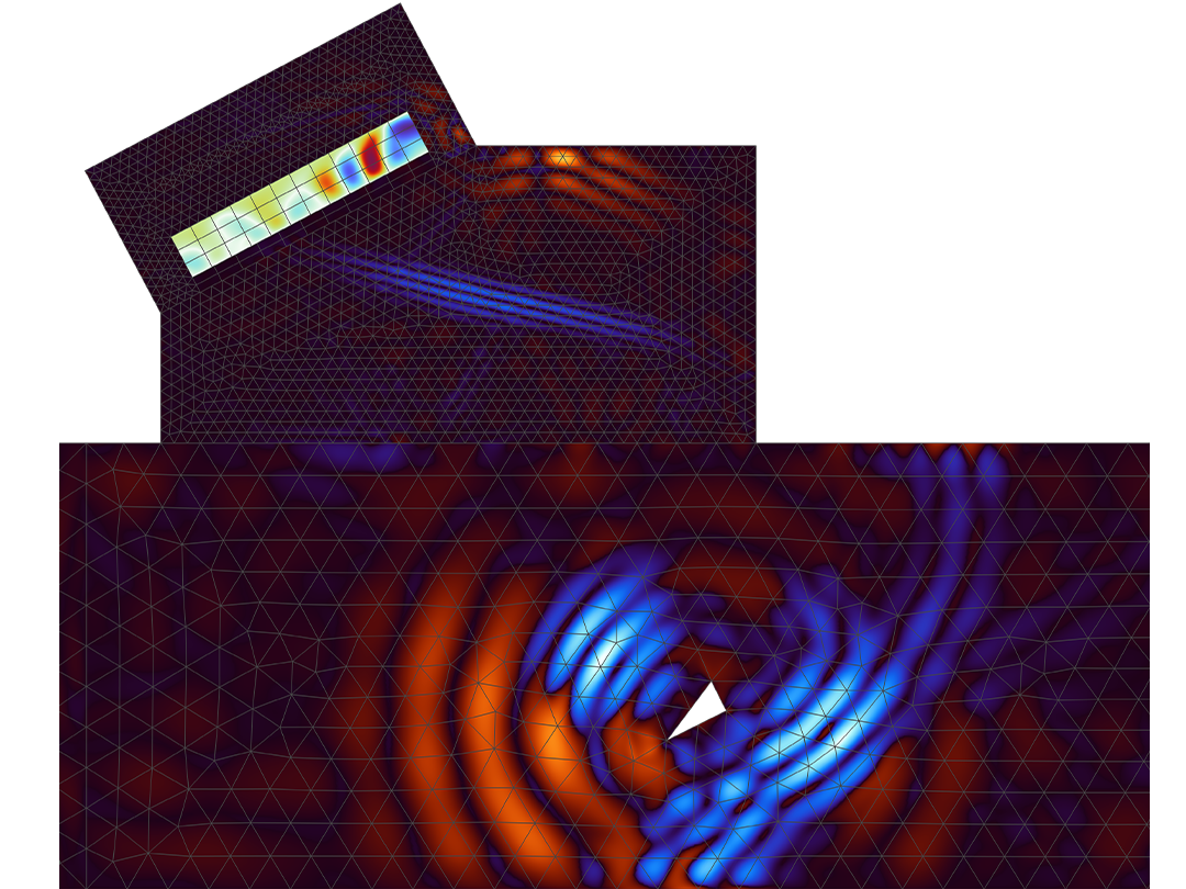
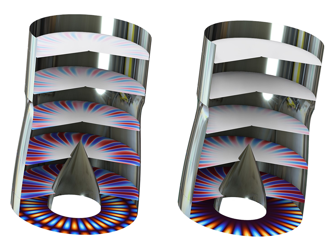
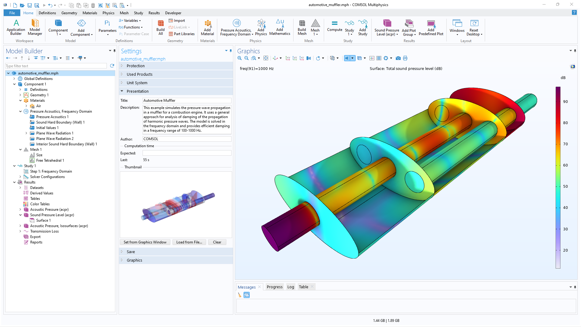
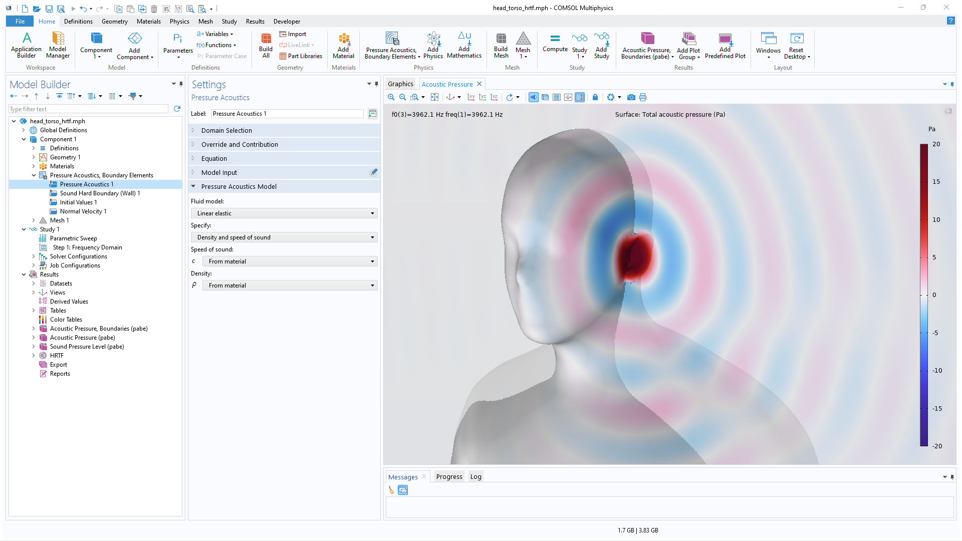
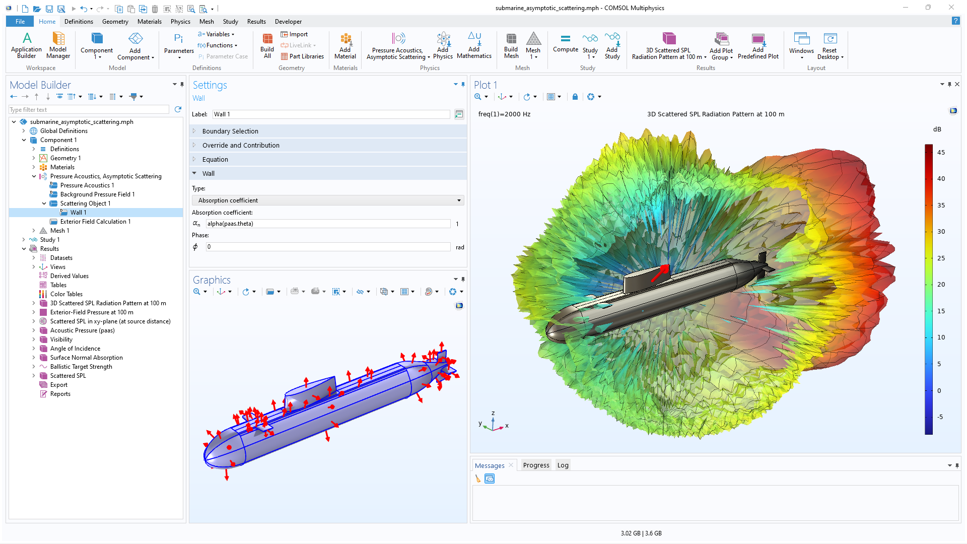
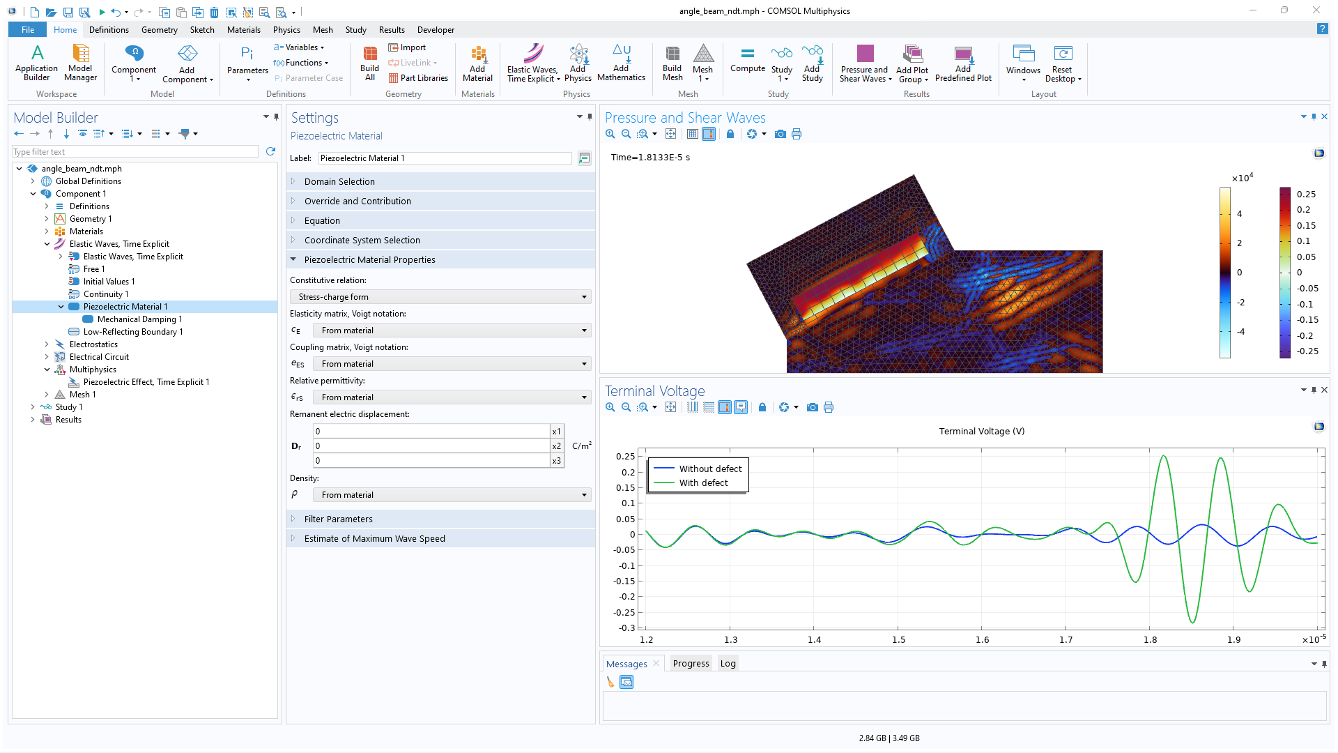
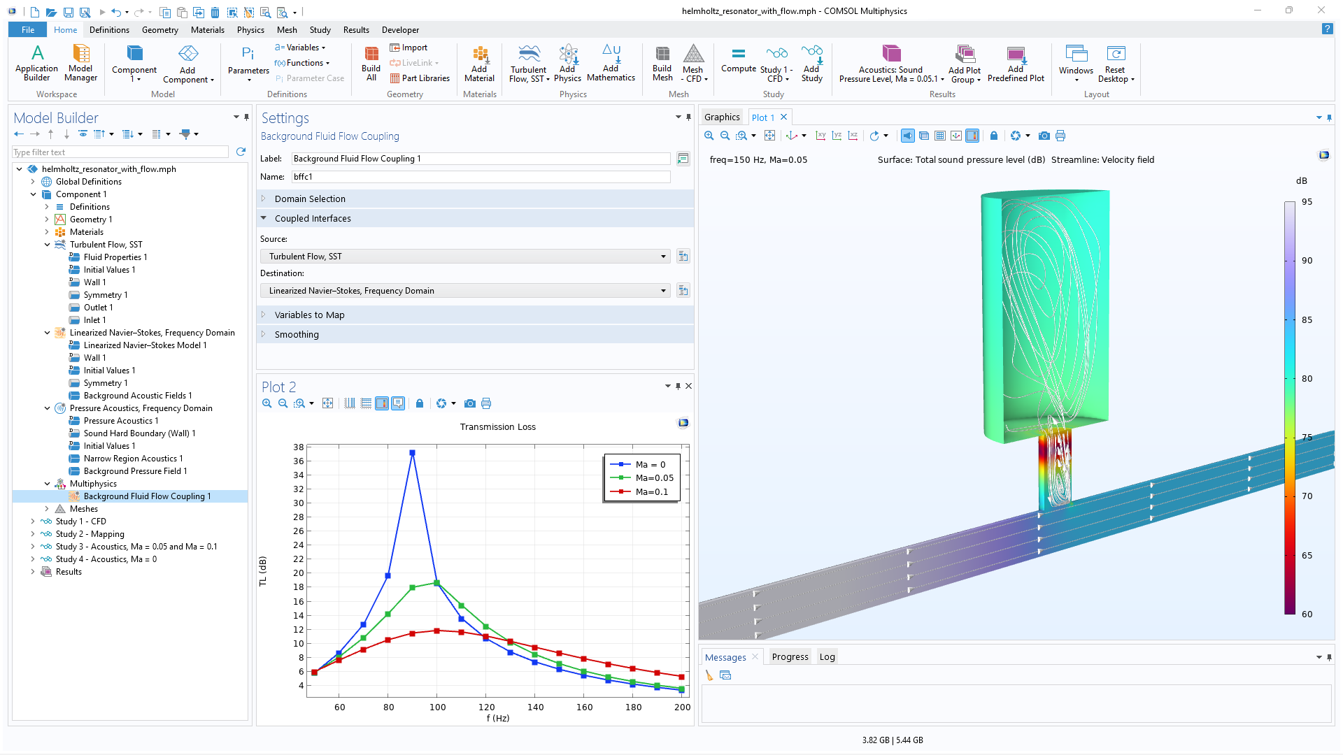
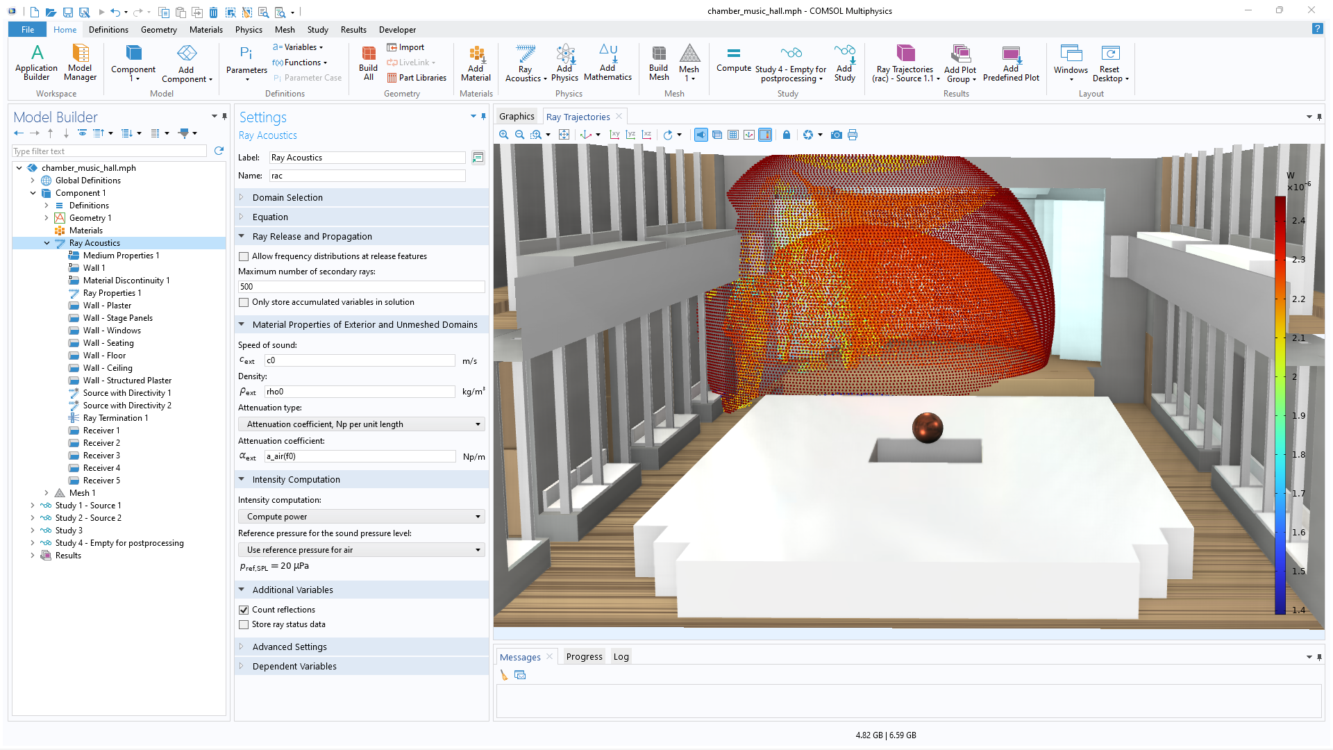
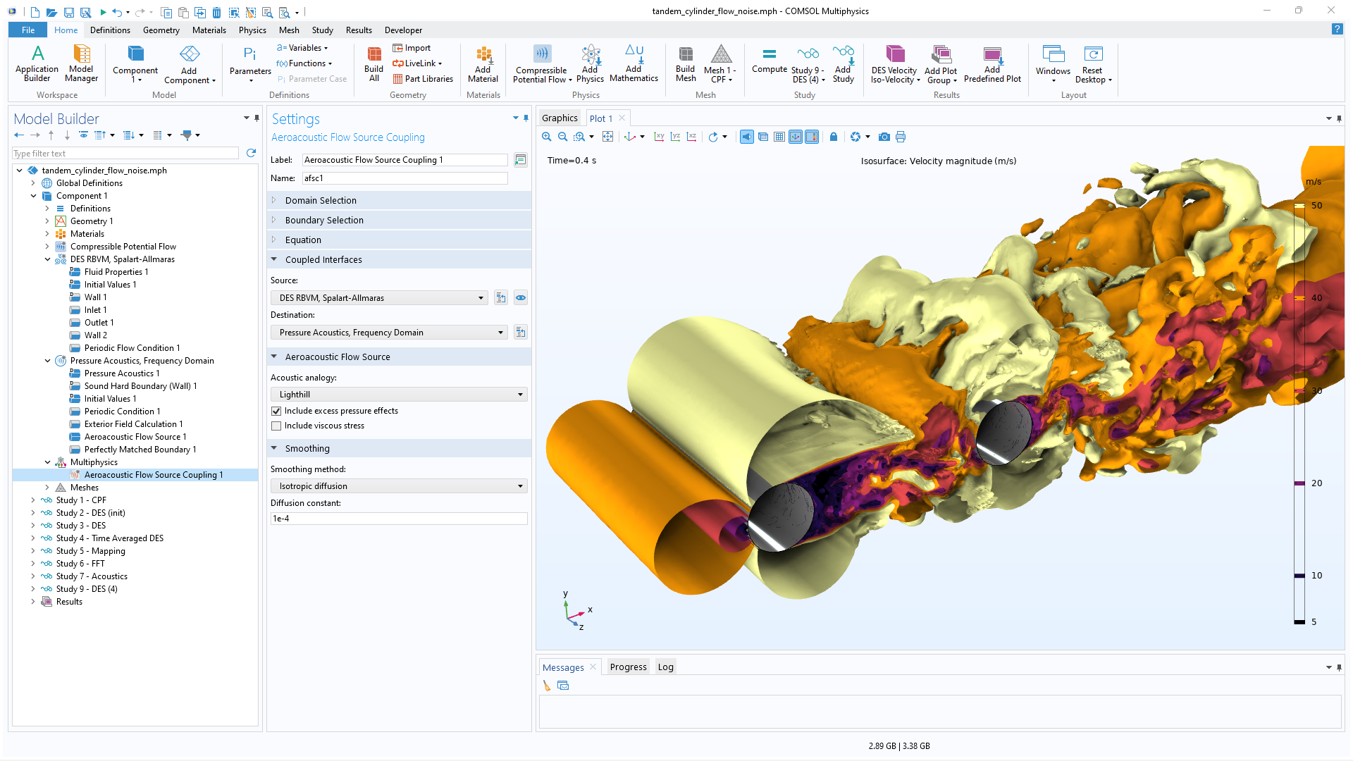
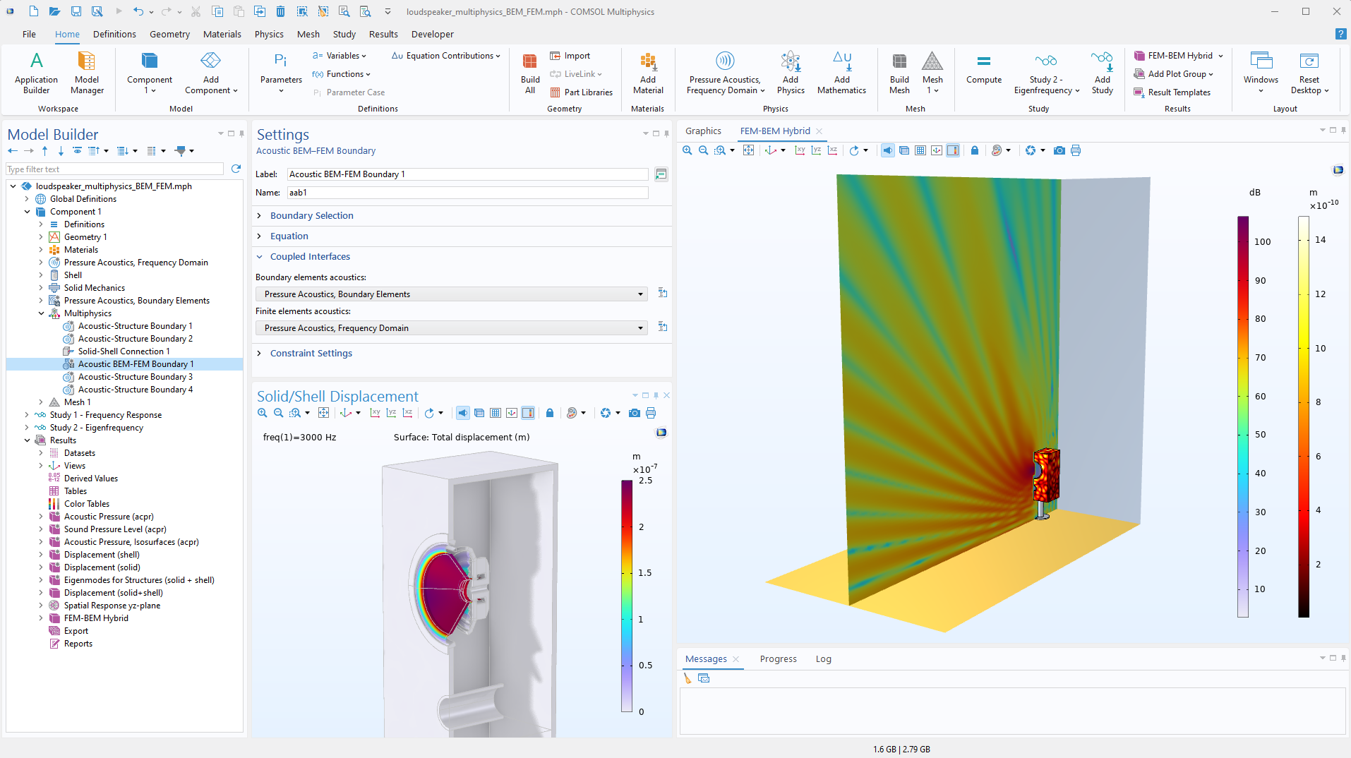
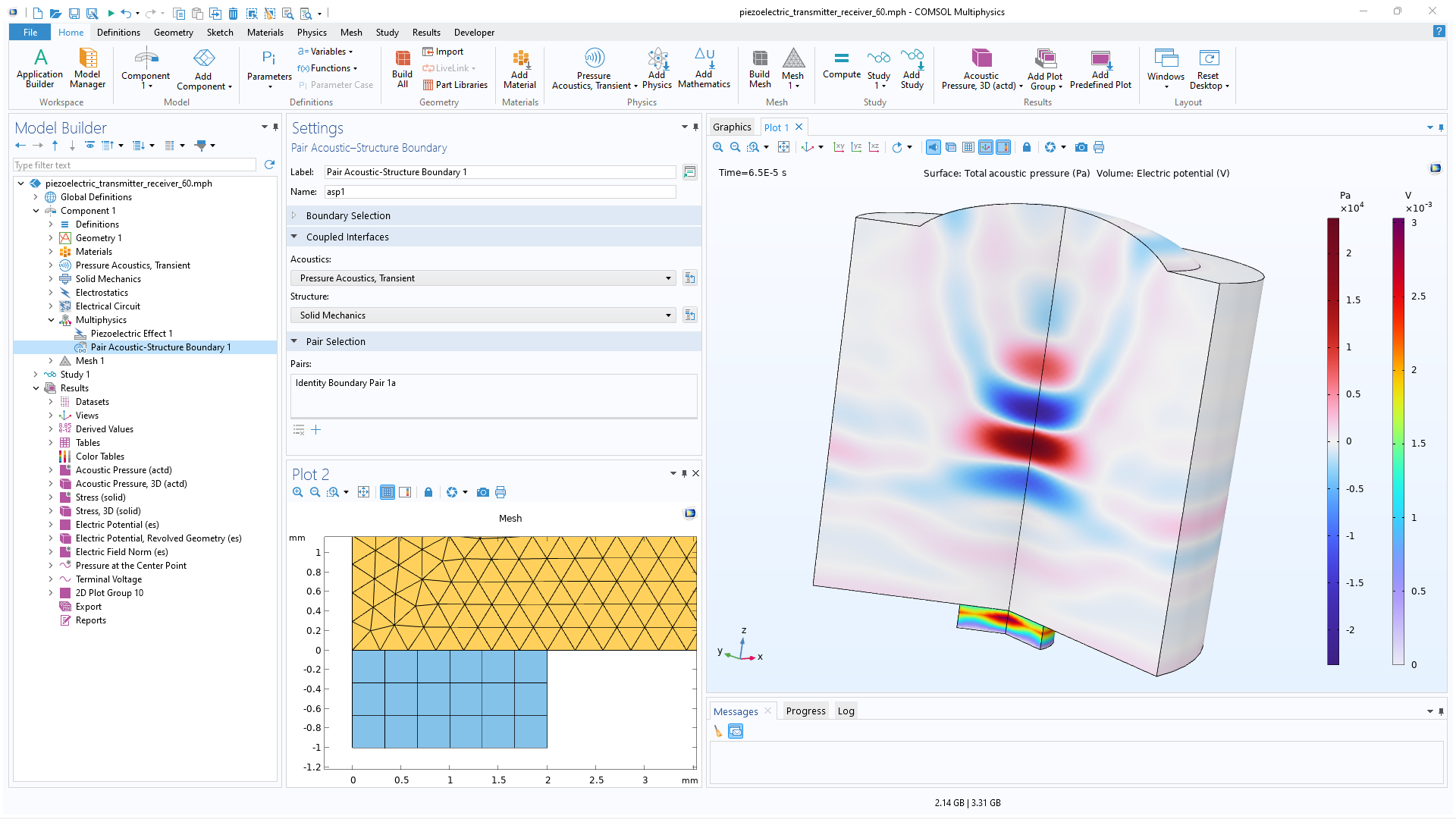
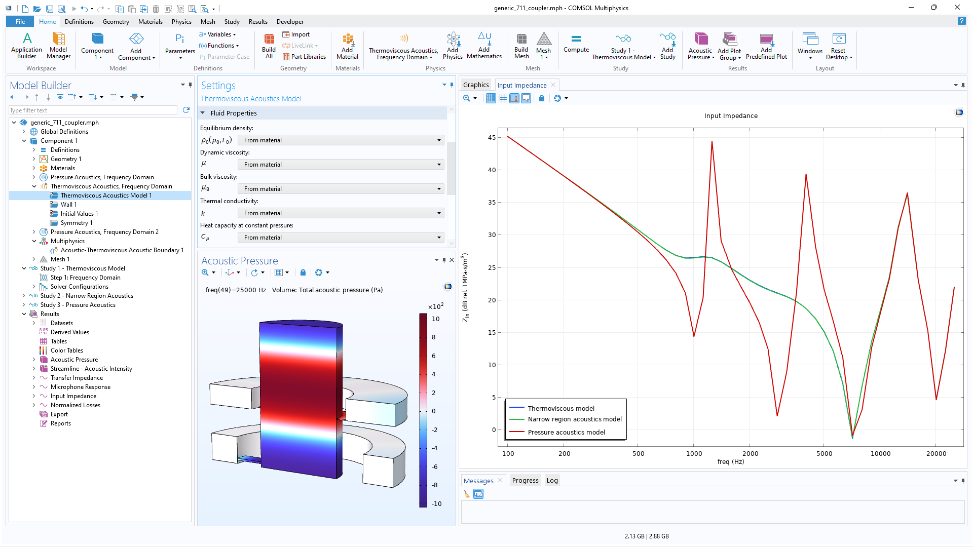
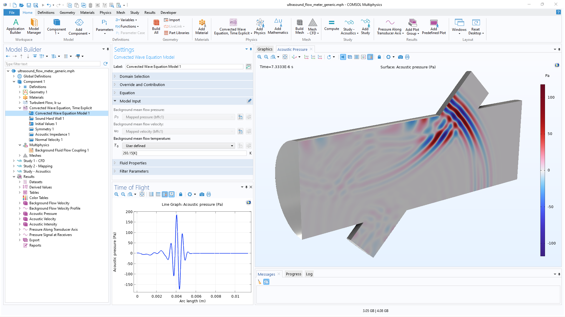
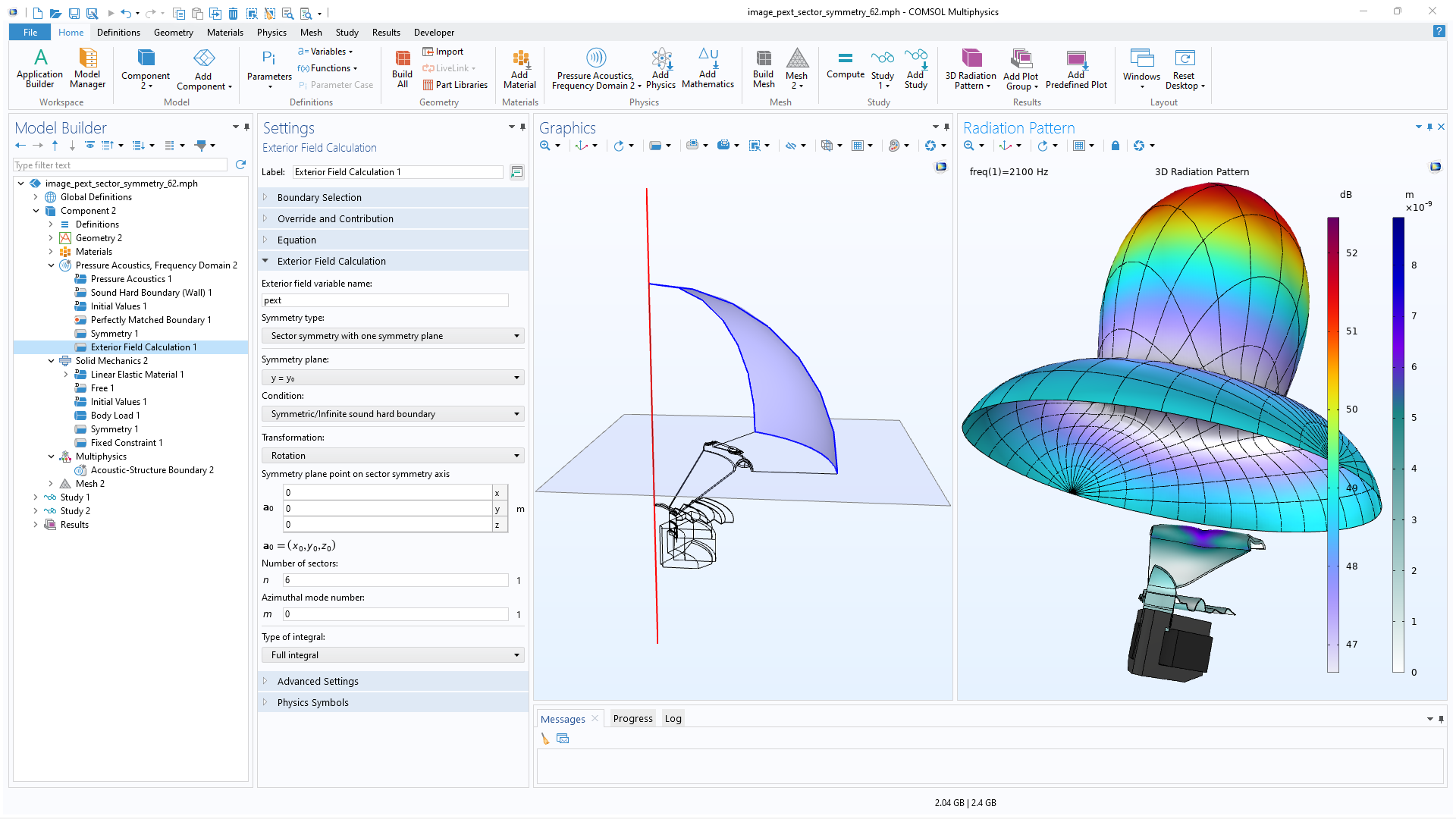
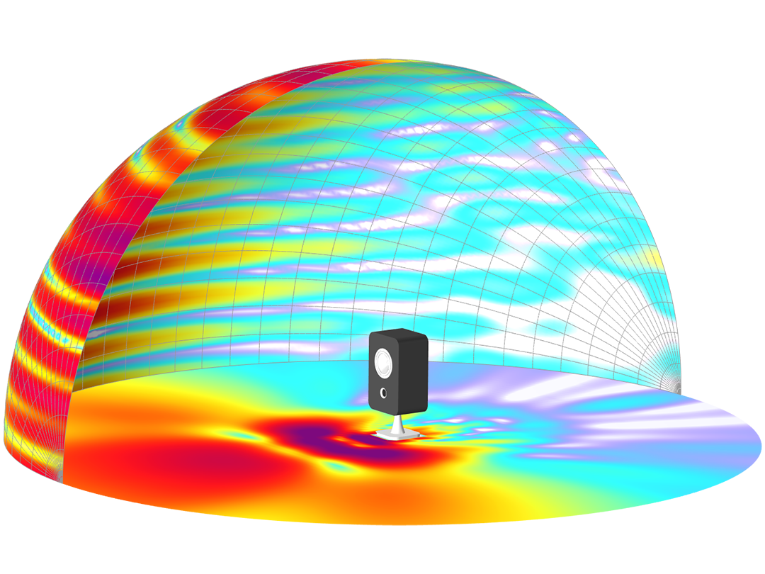
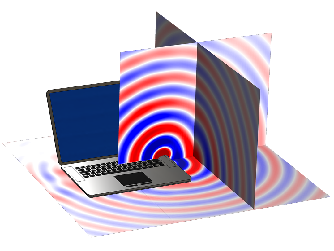
Modeling pressure acoustics is the most common use of the Acoustics Module. The module includes capabilities for modeling pressure acoustics effects, such as the scattering, diffraction, emission, radiation, and transmission of sound. Simulations run in the frequency domain employ the Helmholtz equation, whereas in the time domain, the classical scalar wave equation is used. In the frequency domain, both FEM and BEM are available, as well as hybrid FEM–BEM. In the time domain, time implicit (FEM) as well as time explicit (dG-FEM) formulations are available.

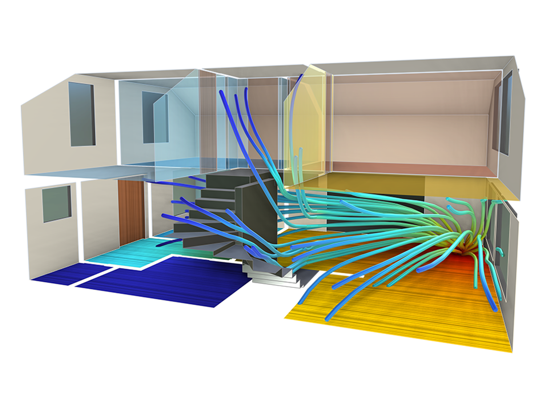
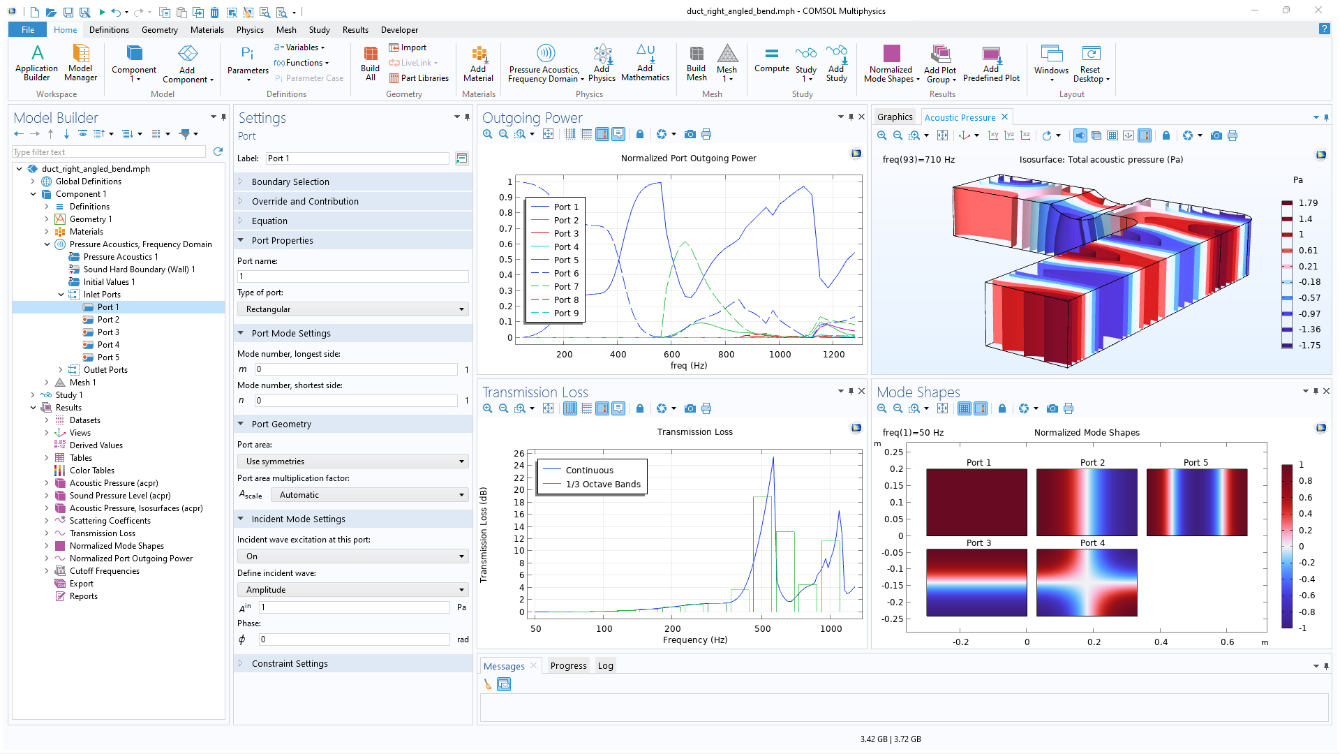
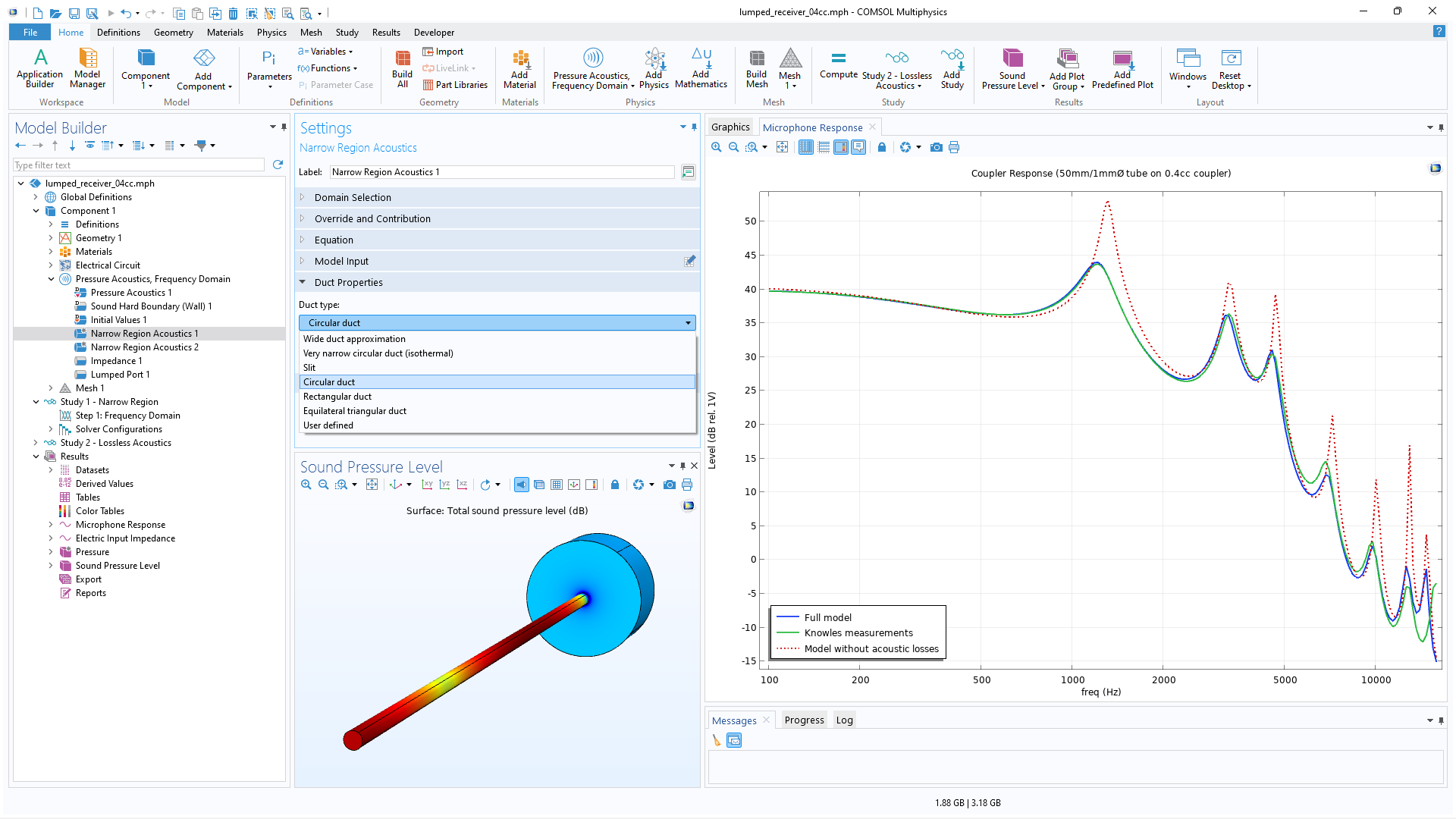
There are many options to account for boundaries in acoustics models. For instance, a boundary condition can be added for a wall, or an impedance condition can be added for a porous layer. Ports can be used to excite or absorb acoustic waves at the inlet and outlet of waveguides using multimode expansion. Sources like prescribed acceleration, velocity, displacement, or pressure can be applied on exterior or interior boundaries. Furthermore, radiation or Floquet periodic boundary conditions can be used to model open or periodic boundaries.
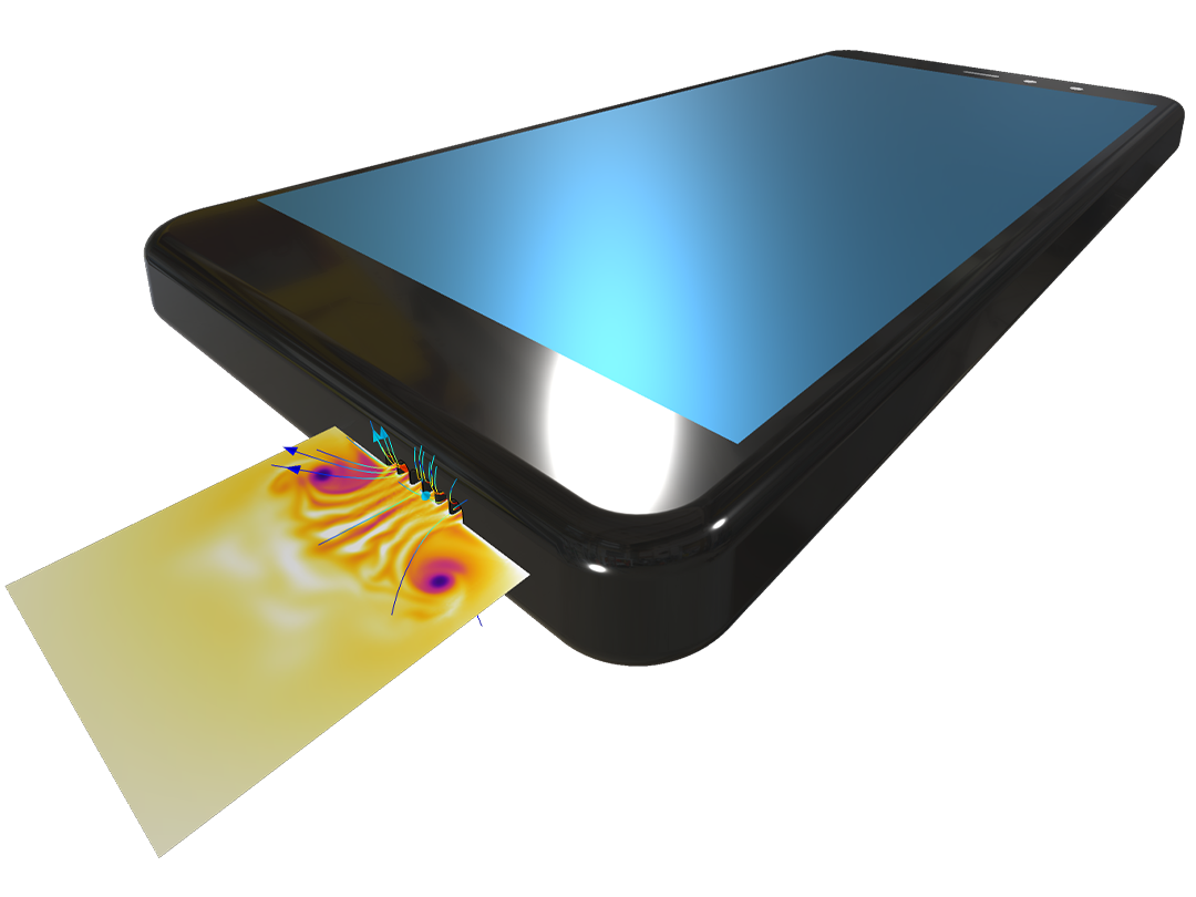
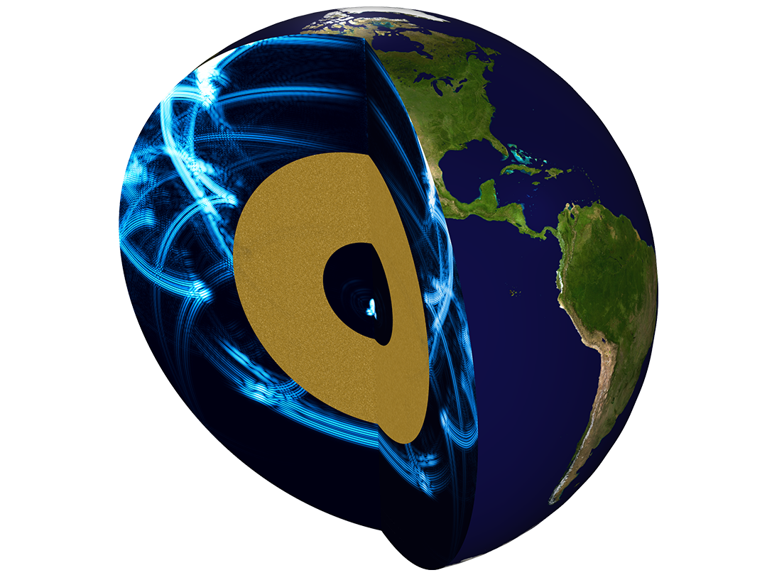
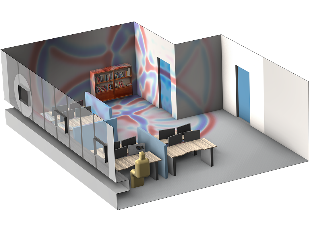
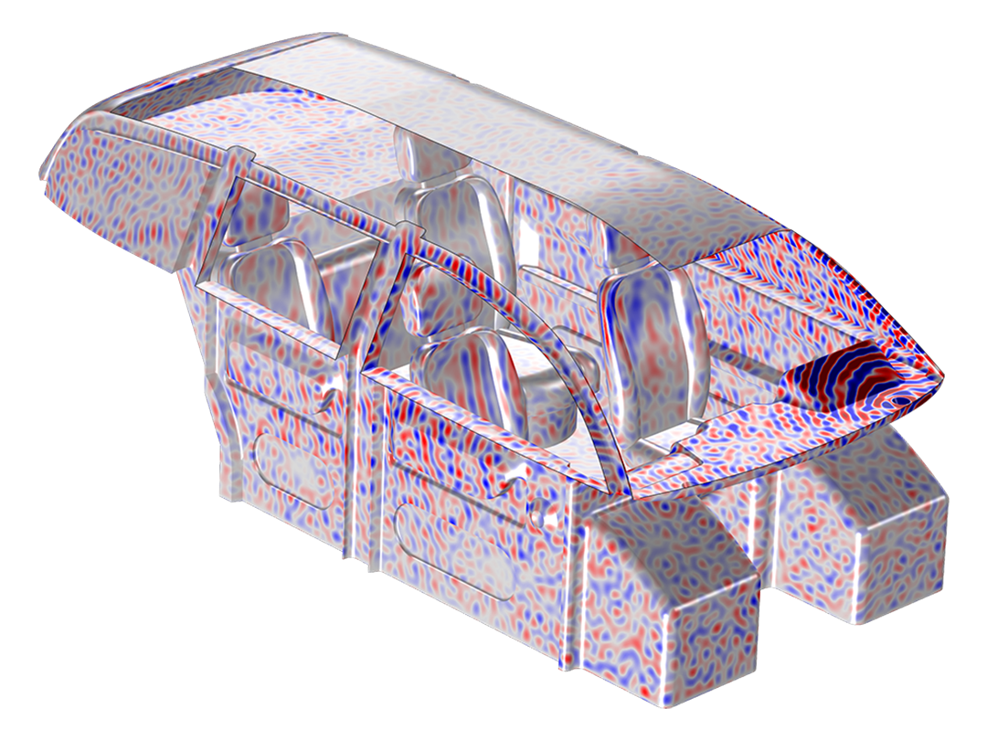
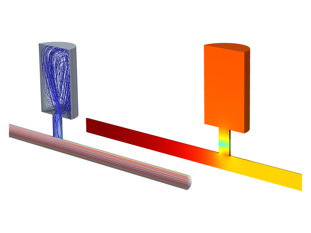
The Acoustics Module can also be used to model pipe acoustics, computing the acoustic pressure and velocity in flexible pipe systems. Applications include HVAC systems, large piping systems, and musical instrument components such as organ pipes.

Electroacoustics: Speakers and Microphones

When modeling speakers and microphones, it is essential to consider acoustic–structure interaction, where the fluid pressure causes a fluid load on the solid domain, and the structural acceleration affects the fluid domain as a normal acceleration across the fluid–solid boundary. The Acoustics Module includes a variety of acoustic–structure interaction capabilities.

For modeling transducers of all sorts, the capabilities included in the Acoustics Module are readily combined with functionality from the AC/DC Module, the MEMS Module, or the Structural Mechanics Module to create fully coupled multiphysics FEM models. This includes detailed modeling of magnets and voice coils in loudspeaker drivers or the electrostatic forces in condenser microphones. In electro-vibroacoustic (i.e., electro-mechanical-acoustic or electroacoustic) transducer systems, it is easy to use lumped circuit models or two-port representations to simplify the electric and mechanical components. Both approaches are solved with a full two-way coupling. There are also features for extracting the lumped representations from full FEM models. In addition, the (linear) small signal behavior and nonlinear large signal dynamics can be modeled and analyzed. In miniature transducer systems, like mobile devices, condenser microphones, and hearing aid receivers, the important damping due to the thermoviscous boundary layer losses is included. There is also extensive functionality for modeling piezoelectric transducers of all kinds.

Microacoustics

For an accurate microacoustic analysis of acoustic propagation in geometries with small dimensions, losses associated with viscosity and thermal conduction need to be accounted for, particularly the losses in the viscous and thermal boundary layers. These effects are solved in full, are automatically included when running a thermoviscous simulation using the Acoustics Module, and are important for vibroacoustics modeling in miniature electroacoustic transducers like microphones, mobile devices, hearing aids, and MEMS devices. In particular, a dedicated acoustic slip-wall condition exists for modeling MEMS devices with very small dimensions or operating a low ambient pressures. For detailed transducer modeling, there are built-in multiphysics couplings between structures and thermoviscous acoustic domains.

The software accounts for additional thermoviscous acoustics physics effects, including the full transition from adiabatic to isothermal thermodynamic behavior at very low frequencies. Local nonlinear effects, such as vortex shedding in microspeaker ports or perforates, can be captured in the time domain with the addition of the nonlinear governing terms.

Elastic Waves and Ultrasound in Solids

The propagation of sound in solids happens through small-amplitude elastic oscillations of the solid's shape and structure. These elastic waves are transmitted to surrounding fluids as ordinary sound waves.

The Acoustics Module can be used to model the propagation of elastic waves in solids and porous materials, for single-physics or multiphysics applications, such as vibration control, nondestructive testing (NDT), or mechanical feedback. Application areas range from micromechanical devices to seismic wave propagation. Elastic wave propagation over large domains containing many wavelengths is solved using a higher-order dG-FEM time-explicit method, and is multiphysics enabled for couplings with fluids as well as piezoelectric materials. The full structural dynamics formulation accounts for the effects of shear waves as well as pressure waves. The coupled propagation of elastic and pressure waves in porous materials solving Biot's equations (the mixed p-u formulation) can be modeled, applicable to both isotropic and anisotropic porous materials.

Ultrasound in Fluids

Acoustic signals with frequencies that are too high to be audible to humans are classified as ultrasound. In fluids, this implies that ultrasonic waves have a short wavelength. Simulating ultrasound in fluids requires computing the transient propagation of acoustic waves in fluids over large distances. With the software, this simulation can be done in two ways: modeling wave propagation that includes a background flow or modeling the effects of high-power nonlinear acoustics.

It is possible to solve for transient linear acoustics in a simulation that contains many wavelengths in a stationary background flow by modeling the convected wave equation. Applications include flowmeters and exhaust systems.

For high-power nonlinear acoustics applications, the software is able to capture progressive wave propagation phenomena where the cumulative nonlinear effects surpass the local nonlinear effects. This includes modeling the formation and propagation of shocks. Applications include biomedical applications such as ultrasonic imaging and high-intensity focused ultrasound (HIFU).

For both options, there are multiphysics capabilities available for fully coupling a model with elastic waves in structures and/or with piezoelectric materials.

Aeroacoustics

Using the Acoustics Module, computational aeroacoustics (CAA) simulations can efficiently be run with a decoupled two-step approach. First, you identify the background mean flow is identified using the CFD Module or a user-defined flow profile; then, you solve for the acoustic propagation is solved for.

For convected acoustics simulations, several finite element formulations are available, including linearized Navier–Stokes, linearized Euler, and linearized potential flow aeroacoustics simulations. There is also support for computing acoustic variations in pressure, density, velocity, and temperature in the presence of any stationary isothermal or nonisothermal background mean flow. The formulations readily account for convection, damping, reflection, and diffraction of acoustic waves by the flow. There is also functionality for FSI fluid–structure interaction analyses in the frequency domain with predefined couplings to elastic structures. Additionally, tools are available for modal source decomposition and for conducting modal transmission loss simulations in the context of duct acoustics, such as those found in turbofan engines.

Flow-induced noise can be included in a pressure acoustics analysis by the addition of aeroacoustic flow sources using Lighthill's acoustic analogy with input from a transient large eddy simulation (LES) or detached eddy simulation (DES) with the CFD model.

Geometrical Acoustics

The geometrical acoustics capabilities of the Acoustics Module can be used to evaluate high-frequency systems where the acoustic wavelength is smaller than the characteristic geometric features. There are two methods available: ray acoustics and acoustic diffusion.

For ray acoustics, the trajectories, phase, and intensity of acoustic rays can be computed. Additionally, impulse responses, energy and level decay curves, as well as the classical objective room acoustic metrics can be calculated. The rays can propagate in graded media, which is necessary in underwater acoustics applications. For simulating ray acoustics in both air and water, specialized atmosphere and ocean attenuation material models are available that are important for wave propagation over large distances and at high frequencies. Additionally, the module features integrated couplings that enable transitioning from wave-based simulation results to ray tracing, enabling the realistic modeling of sources, such as loudspeakers, based on both near-field and far-field computations.

For acoustic diffusion, there is functionality for determining the sound pressure level distribution in coupled rooms and the reverberation times at different locations. The acoustics are modeled in a simplified way using a diffusion equation for the acoustic energy density. This method is well suited for quick analyses inside buildings and other large structures.

Acoustic Streaming

With the Acoustics Module, it is possible to simulate acoustic streaming that describes the physical process where an acoustic field can induce movement in a fluid. The module contains multiphysics capabilities for coupling acoustics and fluid flow with model acoustic streaming phenomena for pressure and thermoviscous acoustics.

Acoustic streaming is a nonlinear phenomenon that occurs due to the nonlinearity of the Navier–Stokes equations. The Acoustics Module computes the forces, stresses, and boundary slip velocities that the acoustic field induces in a fluid in order to generate the streaming flow field. This phenomena is used widely in biotech and semiconductor processing and is important in microfluidics and lab-on-a-chip systems for applications such as particle handling, the mixing of fluids, and microfluidic pumps.

Features and Functionality in the Acoustics Module

Explore the features and functionality of the Acoustics Module in more detail in the sections below.

A close-up view of the Model Builder with the root node highlighted and a muffler model in the Graphics window.

Built-In User Interfaces

The Acoustics Module provides built-in interfaces covering all of the application areas listed above. These interfaces define sets of domain equations, boundary conditions, initial conditions, predefined meshes, predefined studies with solver settings, and predefined plots and derived values. All of the modeling steps performed with these interfaces occur within the COMSOL Multiphysics® environment. Meshing and solver settings are handled automatically by the software, with options for manual editing.

The COMSOL Multiphysics® workflow for building acoustics models with the acoustics interfaces is the same as for building a model with any other physics interface. In this way, it is easy to incorporate multiple physics into one acoustics model, and there are several multiphysics interfaces built into the Acoustics Module and accessible when combining with other add-on modules from the COMSOL product suite.

A close-up view of the Pressure Acoustics node Settings window and a head model in the Graphics window.

Pressure Acoustics Interfaces

For modeling pressure acoustics, there are multiple interfaces where the sound field is represented by a scalar pressure variable. The general-purpose interfaces, based on FEM, include the capability of solving in both the frequency and time domain. For transient models, nonlinear effects can be included and are based on the Westervelt equation.

To efficiently solve large radiation and scattering problems, frequency-domain BEM is available that couples seamlessly with both the acoustic and structural finite-element-based interfaces.

To efficiently solve large transient models, a specialized interface based on the discontinuous Galerkin finite element method and a time-explicit solver is available. This interface can be coupled to the corresponding time-explicit interface for elastic and piezoelectric waves.

A close-up view of the Model Builder with the Wall node highlighted and a submarine model in the Graphics window.

High-Frequency Pressure Acoustics

Two highly specialized interfaces are available for quick high-frequency acoustics analysis in the frequency domain. These interfaces are based on computing the Kirchhoff–Helmholtz integral and include one interface for scattering analysis and another interface for radiation analysis. High-frequency acoustics analysis can be used as a first step before moving on to a more computationally demanding analysis based on FEM or BEM.

A close-up view of the Model Builder with the Piezoelectric Material node highlighted and an angle beam model in the Graphics window.

Elastic Waves Interfaces

The Acoustics Module includes interfaces for modeling the propagation of linear elastic waves in solids, porous, and piezoelectric materials. These interfaces readily couple to fluid domains using a set of built-in multiphysics couplings.

The Solid Mechanics interfaces have the capability of representing full elastodynamics and can be used for modeling elastic waves in solids in both the frequency and time domain. A Port boundary condition is specifically implemented to model and handle various propagating modes in elastic waveguide structures.

The poroelastic interfaces are used for modeling poroelastic waves in porous materials. These waves result from the complex two-way interaction between acoustic pressure variations in the saturating fluid and the elastic deformation of the solid porous matrix. The poroelastic interfaces solve Biot’s equations in the frequency domain and include loss mechanisms from viscous losses (Biot), for modeling rocks and soils, as well as thermal and viscous losses (Biot–Allard), for sound-absorbing materials in air. Models are available for materials with isotropic or anisotropic porous and structural properties, which are relevant in, for example, fibrous porous materials.

Two interfaces, based on a time-explicit discontinuous Galerkin formulation, can be used for modeling linear elastic waves in solid and piezoelectric domains. These interfaces can be coupled and are suited for efficiently modeling domains with several wavelengths. A dedicated Fracture boundary condition can be used to model two solids with nonideal bonding, for example, if the goal is to simulate the acoustic response of a defect or a delamination zone. In addition, these interfaces can be coupled with the time-explicit interfaces for pressure acoustics and the convected wave equation.

A close-up view of the Model Builder and a Helmholtz resonator in the Graphics window.

Aeroacoustics Interfaces

For modeling detailed convected acoustics, or flow-borne noise, a number of aeroacoustics interfaces are available in both the frequency and time domain. These interfaces are used for simulating one-way interaction of a background fluid flow with an acoustic field. There are different physics interfaces that solve the governing equations under various physical approximations.

The Linearized Navier-Stokes interfaces are used for solving for the acoustic variations in pressure, velocity, and temperature.

The Linearized Euler interfaces are used for computing the acoustic variations in density, velocity, and pressure in the presence of a stationary background mean flow that is well approximated by an ideal gas flow.

Special boundary mode interfaces are available for computing propagating and nonpropagating modes in waveguides and ducts in the presence of a background flow. Modal source decomposition and modal transmission loss simulations in duct acoustics, such as turbofan engines, can be achieved using the dedicated port conditions available with the Linearized Potential Flow interface.

For simplified analysis, interfaces for linearized potential flow can be used in both the time and frequency domains.

A close-up view of the Model Builder with the Exterior Field Calculation node highlighted and a loudspeaker model in the Graphics window.

Open Domains and Radiation

To create an open domain in a model, the model can be truncated using so-called perfectly matched layers (PMLs) in both the time and frequency domain. Alternative methods include using radiation boundary conditions or an exterior domain modeled using a boundary element method interface.

For finite-element-based interfaces, an exterior field calculation feature can be used to determine the pressure in any point outside the computational domain. Dedicated results and analysis capabilities exist for visualizing the radiation pattern of the exterior field (near and far field) in polar, 2D, and 3D plots.

A close-up view of the Model Builder with the Aeroacoustic Flow Source Coupling node highlighted and a tandem cylinder model in the Graphics window.

Flow-Induced Noise

Combining the Acoustics Module and the CFD Module results in a hybrid aeroacoustic (CAA) method for modeling flow-induced noise.

The computational method is based on the FEM discretization of Lighthill's acoustic analogy (wave equation). This formulation of the equations ensures that any solid (fixed or vibrating) boundaries are implicitly taken into account.

The functionality relies on coupling an LES or DES fluid flow simulation, using the CFD Module, to an aeroacoustic flow source for pressure acoustics, available in the Acoustics Module.

A close-up view of the Model Builder with the Acoustic BEM-FEM Boundary node highlighted and a loudspeaker model in the Graphics window.

Finite Element and Boundary Element Methods

Most interfaces in the Acoustics Module are based on different versions of FEM. Interfaces based on BEM are available as well, and can be seamlessly combined with FEM-based interfaces. Hybrid FEM–BEM is very efficient for modeling acoustic–structure interaction involving vibrating structures.

Applications for hybrid FEM–BEM include complex geometries of transducers (piezo or electromagnetic) where FEM is used to model the transducer (and its interior) and BEM is used to model the exterior acoustics.

A BEM-based interface can be used to replace an FEM-based radiation condition or PML, as well as the FEM-based exterior-field calculations.

A close-up view of the Model Builder with the Port node highlighted and an angled duct model in the Graphics window.

Boundary Conditions and Sources for Pressure Acoustics

There is a large variety of boundary conditions available for pressure acoustics, including hard walls and conditions for applying sources. There are radiation, symmetry, periodic, and port conditions for modeling open boundaries. Impedance conditions include models for different parts of the human ear and human skin, simple RCL circuit models, and more. Using the interface for boundary mode analysis, allows for studying propagating modes in the cross sections of waveguides and ducts. The options for modeling idealized sources include built-in options for monopole, dipole, and quadrupole point sources.

A close-up view of the Model Builder with the Pair Acoustic-Structure Boundary node highlighted and a transducer model in the Graphics window.

Acoustic–Structure Interaction Interfaces

The interfaces for acoustic–structure interaction apply to phenomena where the fluid pressure causes a load on the solid domain and the structural acceleration affects the fluid domain across the fluid–solid boundary. This is also known as vibroacoustics.

The interfaces include the capability of solving in either the frequency or the time domain. The solids included in the simulations can be isotropic, anisotropic, porous, or piezoelectric.

When the Acoustics Module is combined with the Structural Mechanics Module, the structural side of an acoustic–structure coupling can additionally include structural shells or membranes.

The Acoustics Module can be combined with the Multibody Dynamics Module in order to include the effects of multiple moving rigid or flexible parts connected through various types of joints.

For more advanced options, the Acoustics Module can be combined with the AC/DC Module or MEMS Module to analyze fluid–structure interaction involving electric or magnetic forces, such as in cases where solids have electrostrictive or magnetostrictive material properties.

A close-up view of the Thermoviscous Acoustics Model node Settings window and a 1D plot in the Graphics window.

Thermoviscous Acoustics Interfaces

In order to accurately model acoustics in geometries with small dimensions, it is necessary to include thermal conduction effects and viscous losses explicitly in the governing equations. Near walls, there are viscous and thermal boundary layers. In these layers, viscous losses due to shear and thermal conduction become important because of large gradients.

The interfaces for thermoviscous acoustics include the capability to simultaneously model the effects of pressure, particle velocity, and acoustic temperature oscillations. Thermoviscous acoustics is, for example, used when modeling the response of small transducers like microphones and receivers, also known as microacoustics. A multiphysics coupling with thermoelasticity physics allows for detailed modeling of damping in MEMS applications, including detailed thin-film damping. This functionality is further enhanced with a dedicated acoustic slip-wall condition necessary for systems with very small dimensions or operating at low ambient pressures. The condition should be used for the slip flow regime when the Knudsen number is in the range of 0.001 to 0.1.

The interfaces are available for solving in both the frequency and time domains. In the time domain, nonlinear effects can also be modeled.

Lumped acoustic and electroacoustic representations can readily be extracted from and/or coupled with the computational domain using ports, lumped ports, or the Lumped Speaker Boundary feature. This is useful for system simulation using, for example, the Thiele–Small representation of a microtransducer in a mobile phone.

A close-up view of the Model Builder with the Convected Wave Equation Model node highlighted and an ultrasound flowmeter model in the Graphics window.

Ultrasound and Convected Wave Equation Interfaces

For analyzing transient linear ultrasound devices and processes, there is a convected wave equation interface available. This interface can be used to efficiently solve large transient linear acoustic models containing many wavelengths in a stationary background flow.

For simulating the propagation of high-amplitude nonlinear acoustic waves, a nonlinear pressure acoustics interface is available. This interface includes special functionality for capturing shocks.

Both interfaces include absorbing layers that are used to set up effective nonreflecting-like boundary conditions. The interfaces are based on the discontinuous Galerkin method and use a computationally efficient time-explicit solver.

A close-up view of the Model Builder with the Ray Acoustics node highlighted and a music hall model in the Graphics window.

Ray Acoustics and Acoustic Diffusion Interfaces

The Ray Acoustics interface is available for running simulations in the high-frequency limit, where the acoustic wavelength is much smaller than the characteristic geometric features. In addition, for quick analyses, the Acoustic Diffusion interface is available for solving the acoustic diffusion equation, also known as energy finite elements.

The interfaces for ray acoustics and the acoustic diffusion equation are suited for modeling acoustics in rooms and concert halls. The Ray Acoustics interface can also be used in outdoor or underwater scenarios.

The Ray Acoustics interface is used to compute the trajectories, phase, and intensity of acoustic rays. It includes the capabilities of impulse response analysis, showing the level decay curves and computed objective room acoustic metrics, such as early decay time (EDT), T60 values, etc.

In addition, a set of dedicated features makes it easy to define sources and receivers with spatial directivity. There are also built-in couplings between wave-based simulations of various sources (such as transducers) and ray tracing, which simplify setting up realistic sources based on both the near-field and far-field results.

A close-up view of the Narrow Region Acoustics node Settings window and a 1D plot in the Graphics window.

Acoustic Losses and Porous Materials

A more approximate way of introducing losses is to use the equivalent fluid models available in the Pressure Acoustics interfaces. In a homogenized way, this introduces attenuation properties to the bulk fluid that mimic different loss mechanisms. The fluid models include losses due to bulk thermal conduction, viscosity and relaxation in the atmosphere (air) and the ocean (seawater), as well as equivalent fluid models for simulating the damping in porous materials (in both the rigid or limp regime), such as the Johnson–Champoux–Allard (JCA) model.

In addition to the Thermoviscous Acoustics interface that simultaneously models the effects of pressure, particle velocity, and acoustic temperature oscillations, the Pressure Acoustics interface can also account for thermoviscous boundary layer losses. Narrow-region acoustics can be used in narrow ducts and waveguides of constant cross sections, while the thermoviscous boundary layer impedance (BLI) condition is applicable for geometries larger than the boundary layer.

Every business and every simulation need is different.

In order to fully evaluate whether or not the COMSOL Multiphysics® software will meet your requirements, you need to contact us. By talking to one of our sales representatives, you will get personalized recommendations and fully documented examples to help you get the most out of your evaluation and guide you to choose the best license option to suit your needs.

Just click on the "Contact COMSOL" button, fill in your contact details and any specific comments or questions, and submit. You will receive a response from a sales representative within one business day.

Next Step

Request a Software Demonstration