COMSOL Multiphysics^® 6.3 Release Highlights

Time-Dependent Optimization

The algorithm for gradient-based optimization of time-dependent problems has been improved to use the discrete adjoint method. This works similarly to how all stationary gradient computations are performed in the COMSOL^® software. While the previous continuous adjoint algorithm is still available, this discrete adjoint method is more robust, has better accuracy, and is faster. Note that both algorithms may require recomputation of the forward solution, but the robustness of these restarted computations has been significantly improved. Additionally, the new method provides a speedup equal to the number of measurement points in time when used for parameter estimation with the interior point optimizer (IPOPT) or sparse nonlinear optimizer (SNOPT) optimization solver.

Advanced settings for gradient-based optimization of time-dependent problems can be accessed by selecting Adjoint as the gradient method for the Optimization Solver. The default settings are robust, so adjustments are typically unnecessary and offer little additional benefit.

Efficient Global Optimization

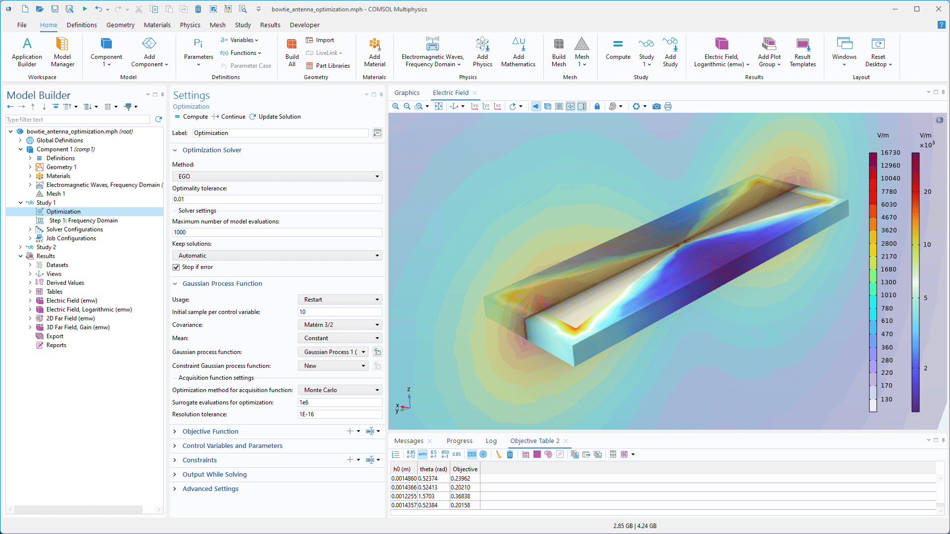
The efficient global optimization (EGO) solver has been added as a new gradient-free optimization solver to the Optimization study step. This solver uses Bayesian optimization to construct a surrogate model that emphasizes accuracy in areas with good objectives. The local solvers in previous versions — such as the bound optimization by quadratic approximation (BOBYQA) solver — are faster than this solver; however, in some cases, the EGO solver consistently identifies better objective values. The EGO solver requires bounds on the control parameter, but initial values and scales are not used. It is possible to inspect the Gaussian response surface after the optimization, which can be helpful in evaluating how sensitive the objective is to perturbations in different regions. The solver shares functionality and settings with the Uncertainty Quantification Module but only requires a license for the Optimization Module.

The EGO solver is available for the Optimization study step. Increasing the number of initial samples per control variable can improve the likelihood of identifying the global optimum. The result can be further improved by switching to another (local) gradient-free solver and continuing the optimization by using the Continue button in the Settings window.

Eigenvalue Optimization

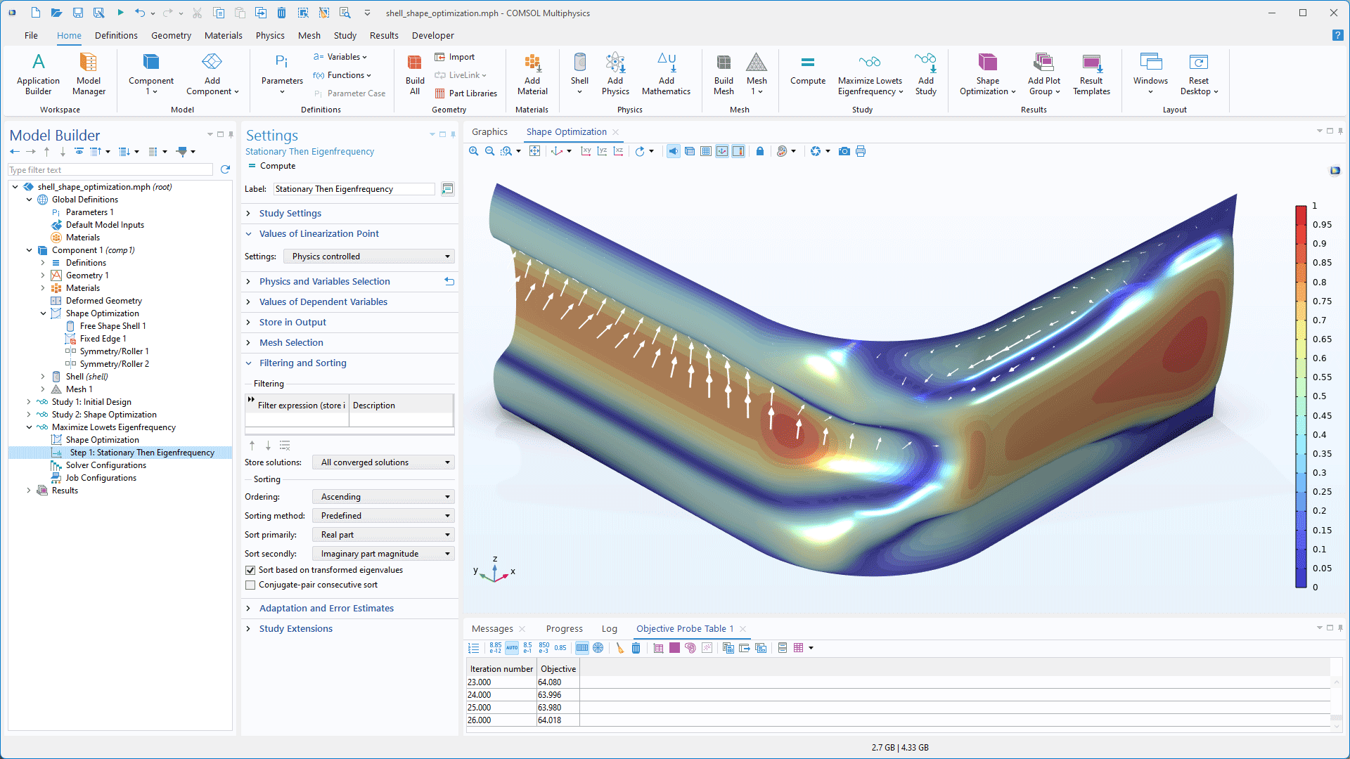
In version 6.3, support for nonlinear eigenvalue problems has been added and is compatible with existing features for eigenvalue optimization, including the Stationary Then Eigenfrequency study step. There are also new tools for sorting and filtering of the eigenvalues, which can be useful in the context of optimization.

The settings for sorting and filtering of eigenvalue solutions are available for several study steps, including the Stationary Then Eigenfrequency study step.

Discrete Adjoint Solver Type

A new Time discrete adjoint solver type is available for optimal control and time-dependent parameter estimation. This solver type is based on a discrete sensitivity method, which provides enhanced robustness, improved accuracy, and faster performance for gradient-based optimization with the Time-Dependent Solver.

In transient parameter estimation problems, significant speed improvements are achieved with the SNOPT or IPOPT solvers. This acceleration is due to the aggregated sensitivity of the entire objective being computed in a single pass instead of separate calculations being made for each measurement point. The previous continuous sensitivity method is still available, but it is no longer the default for transient optimization.

Both the discrete and continuous methods reduce memory consumption through checkpointing, which involves recomputation of the forward solution. In addition, there is a new Out-of-core option that can alternatively be used for forward solution handling, which instead uses temporary disk space to avoid recomputation.

Settings for the Shape Optimization study step using a Time Dependent study step for the optimization of a chemical etching process where the objective is obtaining a symmetric trench as a result of the etching.

Miscellaneous Improvements

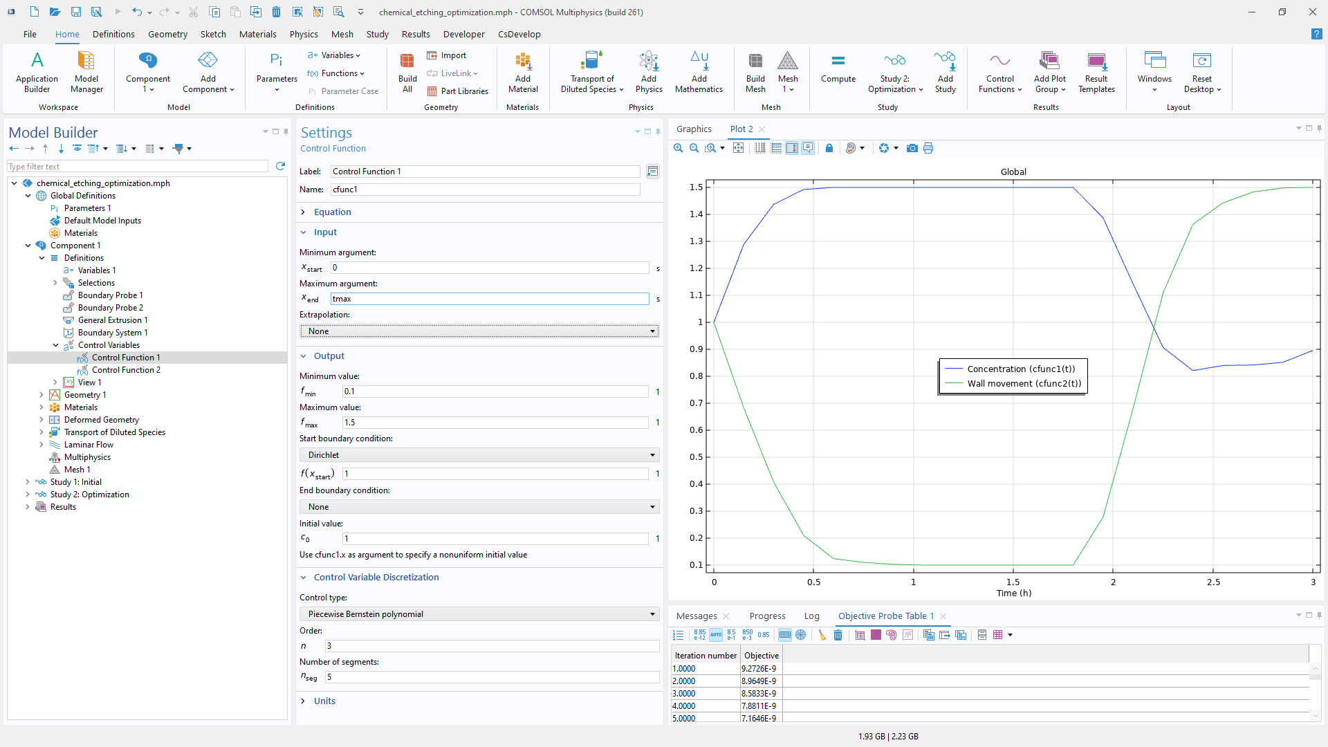
In previous versions, the Free Shape Boundary and Free Shape Shell features supported preserving the continuity of the normal across all or no symmetry boundaries. In this version, these features have been updated, and it is now possible to select which boundaries to preserve the symmetry for. The Polynomial Boundary and Polynomial Shell features have also been updated to include support for preserving the normal at fixed edges in 3D. Additionally, the Control Function feature has been improved with support for a nonuniform initial value and a redesigned user interface. Finally, the Global Least-Squares Objective feature has been moved to Global Definitions.

The Control Function feature now supports physical quantities, a nonuniform initial value, and extrapolation settings.

New Tutorial Models

COMSOL Multiphysics^® version 6.3 brings several new tutorial models to the Optimization Module.

Pyrolysis of Wood with Time-Integrated Objective

Pyrolysis of wood is a process that intrinsically involves multiphysics.

Application Library Title:
pyrolysis_wood_odeobj
Download from the Application Gallery

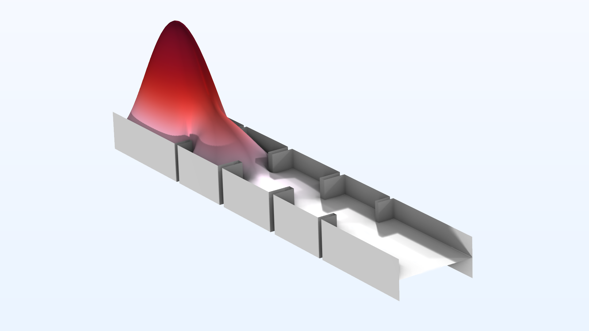
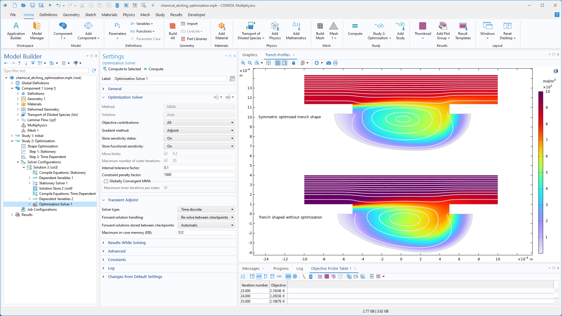
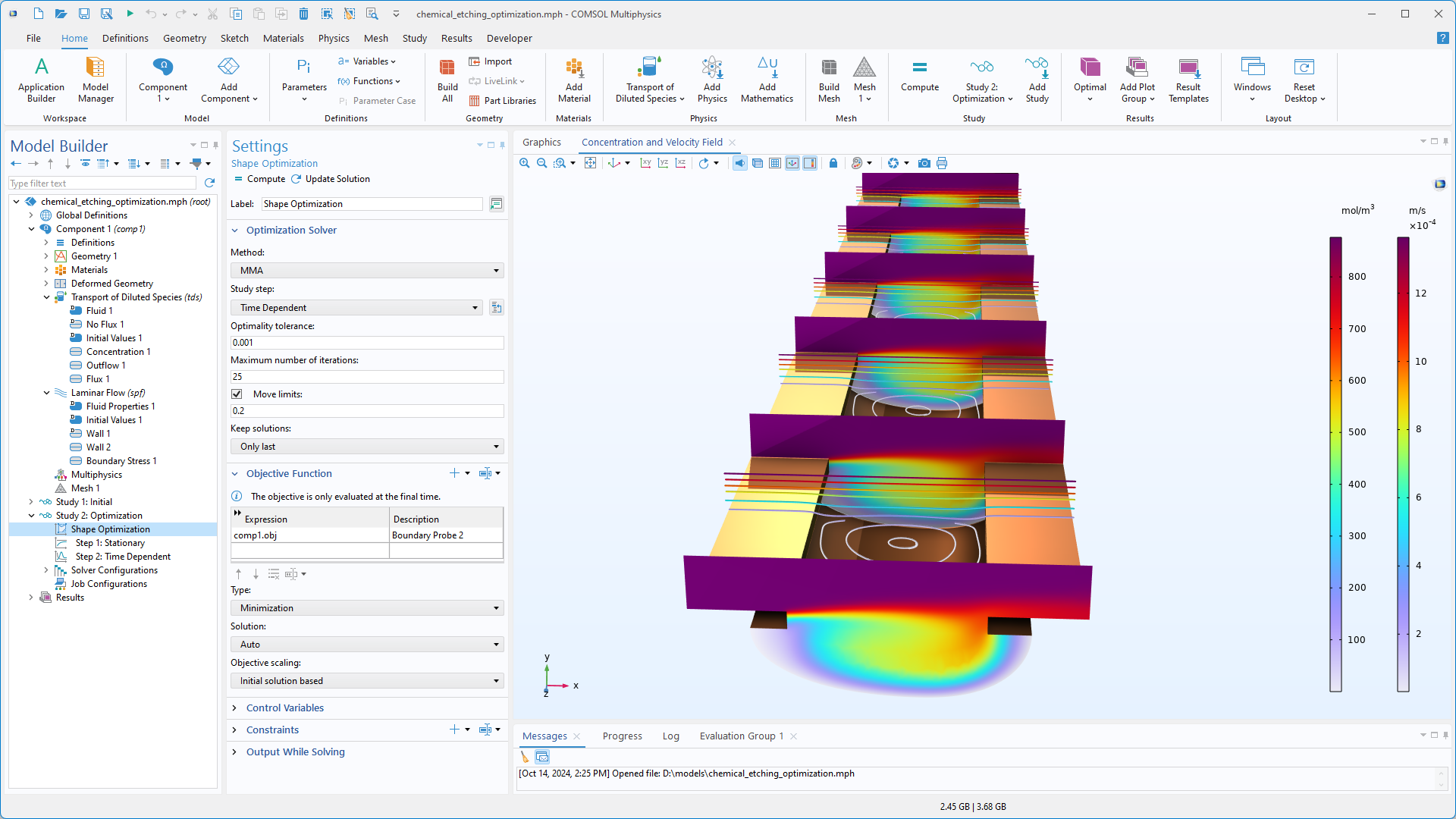
Optimization of Chemical Etching

The etching profile is shown before (left) and after (right) optimization. Both results also show the flow velocity and chemical concentration at the final time.

Application Library Title:
chemical_etching_optimization
Download from the Application Gallery

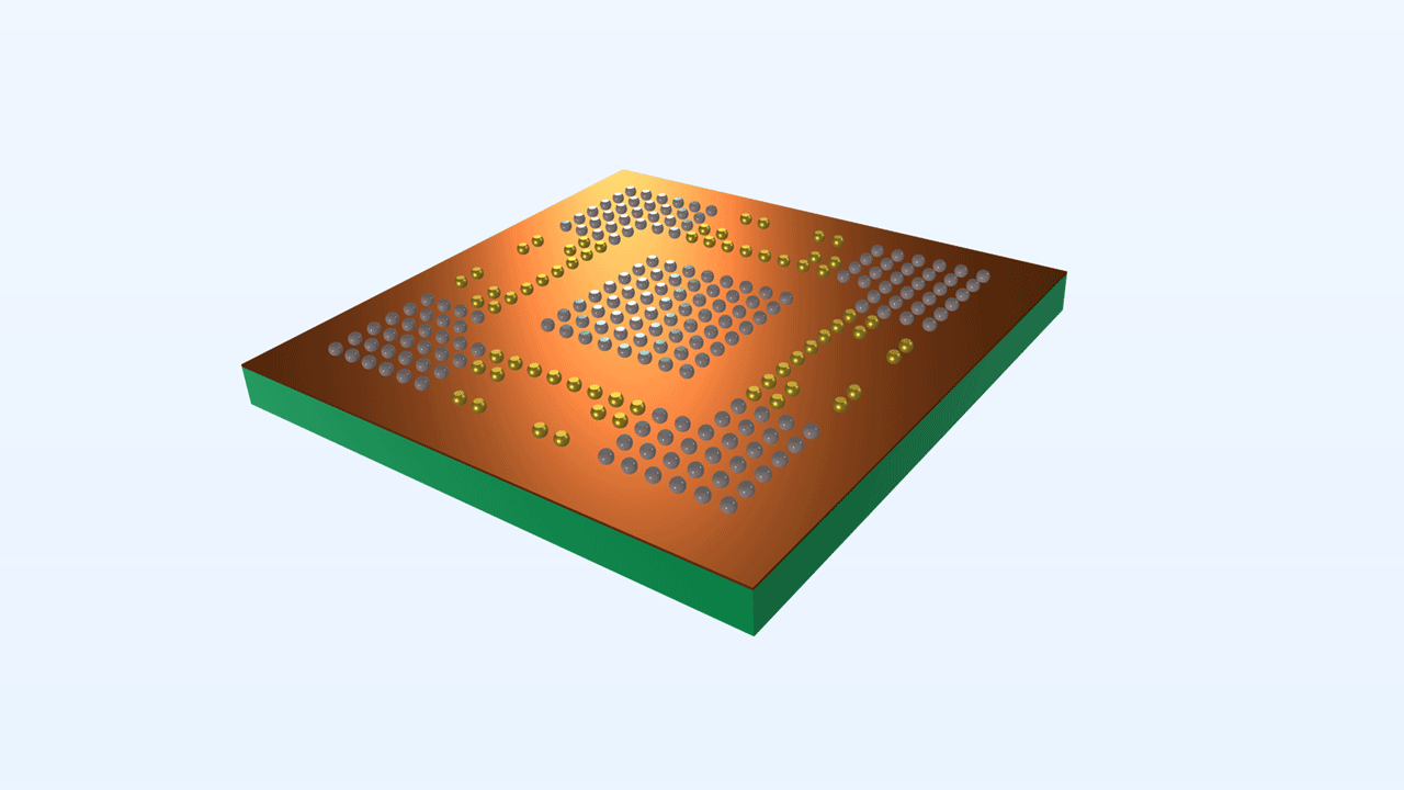
Optimization of the Solder Ball Array to Minimize Chip Warpage

The ball grid array (BGA) technology is a surface-mount technology widely used in electronic packaging. Usually, there are two types of solder balls considered in the array, including the functional balls that are required for electric connections and the support balls that are used for reinforcement only. In this model, the placement of the support solder balls in the array is optimized to minimize the warpage of the chip during operation.

Download from the Application Gallery

Bow Tie Antenna Optimization

A finalized bow tie antenna geometry after using the EGO optimization solver.

Application Library Title:
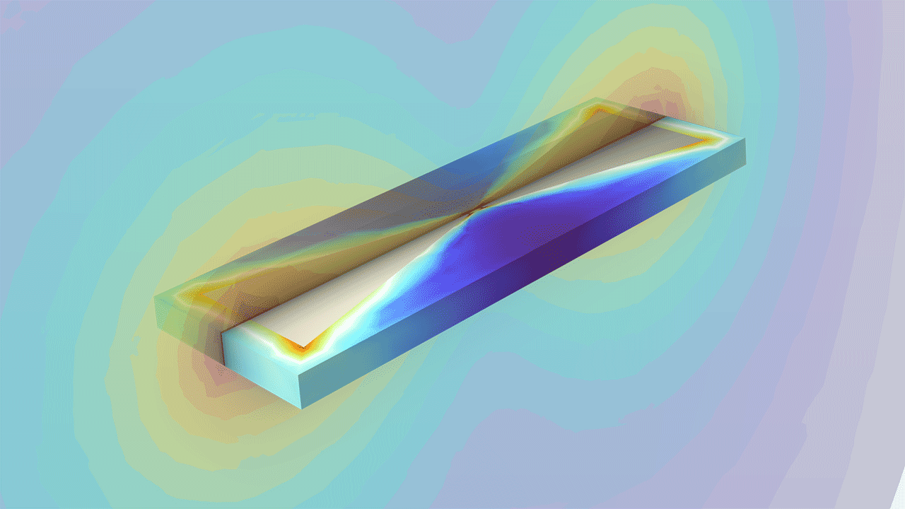
bowtie_antenna_optimization
Download from the Application Gallery

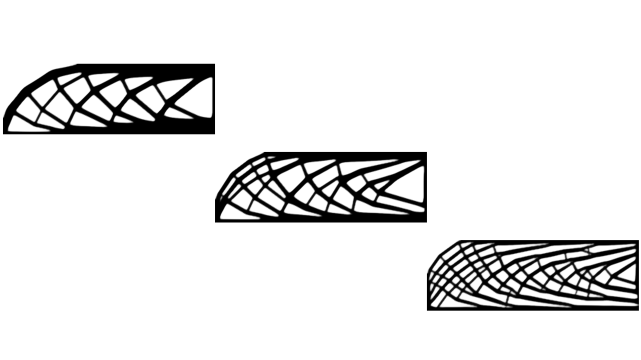
Topology Optimization of an MBB Beam with a Maximum Length Scale

Thick member sizes can cause problems for some manufacturing processes. This model demonstrates how the existing topology optimization features can be extended to accommodate a maximum length scale.

Download from the Application Gallery

Optimization of a Waveguide Iris Bandpass Filter — EGO Version

The magnitude of the electric field is plotted in the optimized geometry for one of the frequencies that should be rejected by the filter.

Download from the Application Gallery